Author: ramzy

  • Reading a Boring Log for Helical Pile Design: A Worked Example

    Reading a Boring Log for Helical Pile Design: A Worked Example

    Take the bearing stratum depth and N-value off the log, correct N for hammer energy and overburden, convert to a friction angle, compute effective overburden stress at each helix using buoyant unit weights, and sum Ah·q’·Nq across the plates. Divide the required ultimate by Kt and you have the installation torque to write on the drawing.

    That is the workflow, and it is not just convention — it is IBC §1810.3.3.1.9, which sets the allowable axial load of a helical pile at Pa = 0.5 Pu (Equation 18-4) and defines Pu as the least of several quantities, the first being the sum of the areas of the helical bearing plates times the ultimate bearing capacity of the soil. Florida adopts the model IBC deep-foundation provisions through the Florida Building Code. The factor of safety of 2 you have seen your whole career is that 0.5.

    This post runs the method end to end on a realistic west-central Florida profile. The first configuration we try fails by a factor of two. The second one gets within a percent and a half of passing — and still fails, on every assumption we test it against. Only the third works. That sequence is the useful part. A clean worked example teaches you the arithmetic; a failed one teaches you where the arithmetic bites.

    We build both the rigs that produce these logs and the piles designed from them, which is the only reason we can write this particular post.

    What a pile designer actually uses

    Column What it’s for
    Depth and layer boundaries Sets helix elevations, defines top and bottom of the bearing stratum
    N-value — all three 6-inch increments Source of φ and Su. Never use only the summed N; the increments reveal shell and gravel spikes and weight-of-rod zones
    USCS symbol and description Decides whether you’re on the drained branch (φ, Nq) or the undrained one (Su, Nc = 9)
    Groundwater — at drilling, at 24 hours, seasonal high Effective overburden. In sand this drives capacity directly
    Sample recovery Zero recovery is data — raveling, running sand, or a void
    Drilling notes Fluid loss and “fell by weight of rod” are karst indicators
    Termination depth A hard constraint. You cannot design a helix below the depth you explored

    Largely ignored for capacity: moisture content, Atterberg limits except to pick a correlation and flag organics, and the minus-200 fraction beyond classification.

    What makes a stratum worth bearing in

    Worth separating what the code says from what is judgment, because most published lists blur them:

    Criterion Value Status
    Allowable load = half the ultimate Pa = 0.5 Pu Code — IBC §1810.3.3.1.9, Eq. 18-4
    Firm soil for bearing and lateral support N ≥ 5 Code-adjacent — AC358 §3.11.2.1 defines firm N≥5, soft 0<N<5, fluid N=0
    Practical minimum for a helix bearing layer N ≥ 10–15 sand, 8–10 clay Judgment — in no code
    Inter-helix spacing 3 × diameter of the lower plate Industry practice — stated in the ESRs, not in the IBC. AC358 Table 3 sets 2.4D–3.6D as the conformance window for using the default Kt
    Pile-to-pile spacing before group effects 3D clear / 4D center-to-center Code-adjacent — AC358 §6.7 (this is the pile spacing rule, often misquoted as the helix rule)
    Uppermost helix depth in tension ≥ 12 × largest helix diameter Code-adjacent — AC358 §4.4.1.1, §6.9, tension only
    Bearing layer thickness below the lead helix ≥ 3 × helix diameter commonly cited Judgment — no code number exists
    Depth for “deep” bearing behavior > 5 × largest helix diameter Practice
    Same bearing layer present in every boring — Judgment, and the most violated rule

    Three borings, one site, three different answers

    Before any arithmetic, the thing that should worry you most. These are real borings from a City of Tampa project, all on one site:

    Depth 16–20 ft B-01 B-02 B-03
    Material Soft clayey weathered limestone No recovery Soft sandy clay
    N-value 12 5 12, then 4

    At the depth where you would want your helix, one boring found weathered limestone, one recovered nothing at all, and one found soft clay that gets softer. A design tuned to B-01 could be off by a factor of three at the pile nearest B-03.

    Another regional example: two adjacent borings where the top of weathered limestone varied from 18.5 ft to 28.5 ft — a ten-foot swing between neighbors.

    This is the Florida condition, and it is why “we have a boring log” and “we have a design basis” are not the same sentence.
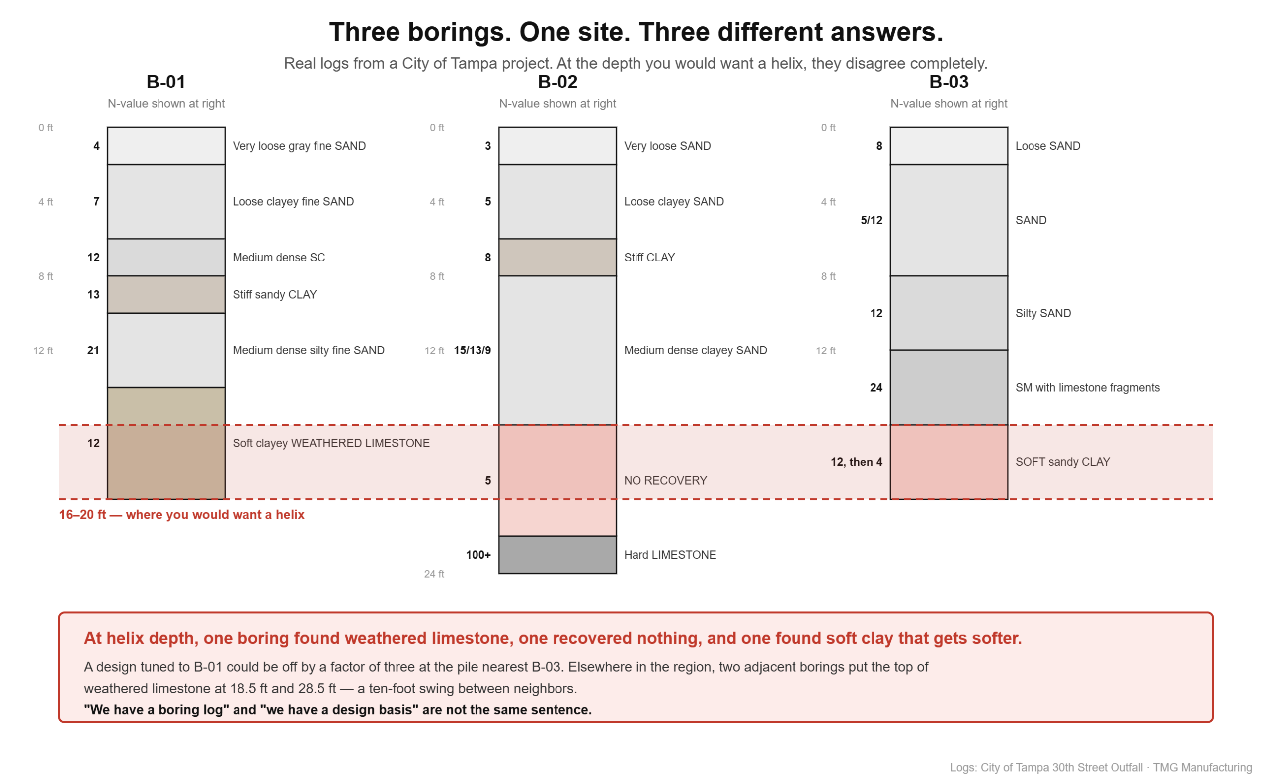
    Three borings from one City of Tampa site. At the depth you would want a helix, they disagree completely.

    From N-value to soil parameters

    Correct N first

    Published correlations are written for N60 — N corrected to 60% hammer energy. Field N is not N60.

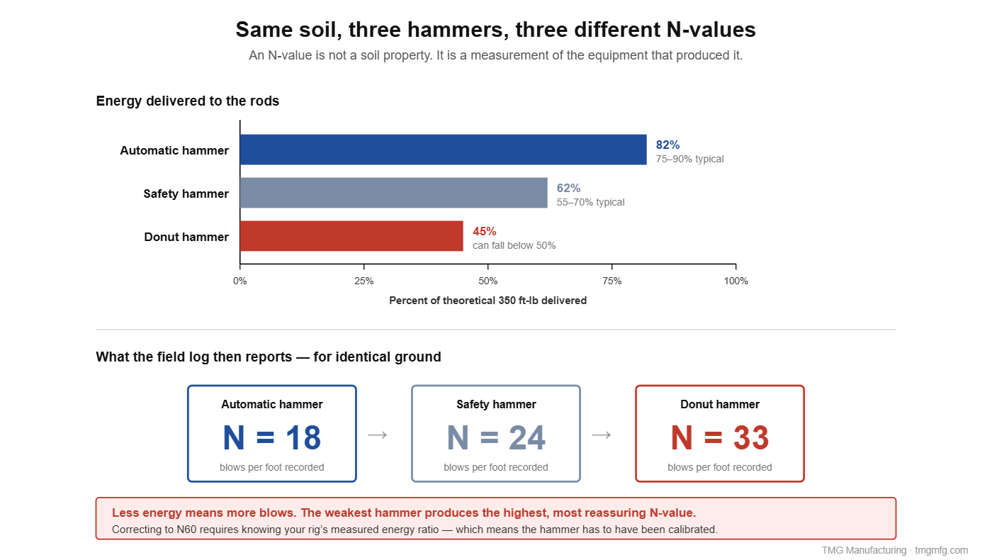
    N60 = N × (hammer efficiency / 60), with adjustments for borehole diameter, sampler, and rod length. Automatic hammers commonly run 75–85% efficiency; safety hammers 55–60%.

    The correction does not always go up. An automatic hammer at 80% turns a field N of 25 into N60 ≈ 33 — a 33% increase. A safety hammer at 55% turns that same field N of 25 into N60 ≈ 23 — a decrease. Which direction you move depends entirely on the hammer, and the hammer is in the report’s methodology section, if it is stated at all. Assuming every correction is upward is how you end up unconservative on a safety-hammer log. (We wrote a whole post on why that number moves so much.)

    For granular soils you then normalize for overburden: CN = √(Pa/σ’v0), giving (N1)60. Because Florida water tables are shallow, effective stress is low and CN often lands between 1.3 and 1.7 at helix depth — a large upward correction.

    Then convert — and look at the spread

    At our example point — field N = 25, safety hammer taken at 60% so N60 = 25, effective overburden 1,058 psf, giving CN = 1.41 and (N1)60 = 35:

    Correlation Argument φ
    Peck-Hanson-Thornburn (Wolff 1989 fit) (N1)60 = 35 37.0°
    Peck-Hanson-Thornburn (Wolff 1989 fit) N60 = 25 34.3°
    Industry helical correlation, φ = 0.28N + 27.4 N = 25 34.4°
    Hatanaka & Uchida (1996), φ = √(20·(N1)60) + 20 (N1)60 = 35 46.6°
    Kulhawy & Mayne (1990) N60 = 25, σ’v/Pa = 0.50 46.1°

    A 12-degree spread from one N-value. Because Nq is exponential in φ, going from 34° to 46.6° is a factor of more than five on computed helix capacity. Note also that Hatanaka & Uchida is defined on (N1)60, not N60 — feeding it raw N60 is a common error that lands you about 4° low and quietly looks reasonable.

    Hatanaka & Uchida and Kulhawy & Mayne are known to run high for fine, rounded, uniform quartz sands — which is exactly what Florida has. Most Florida practitioners cap φ at 32–35° for medium dense fine sand regardless of what the correlation returns. That cap is judgment, not derivation, and anyone presenting it as a calculation is overselling it.

    We will design at φ = 34°, the value the two conservative correlations agree on. Note what that means: we normalize N for overburden to see the spread, then design off the un-normalized branch. That is deliberate and conservative — using (N1)60 = 35 would give φ = 37° and about 46% more capacity — but it should be stated, not buried, because a reviewer will ask which one you used.

    For clays, Su ≈ 125·N psf is the traditional relation. Treat it with real suspicion. Reid and Taylor’s re-analysis of the underlying dataset (Ground Engineering, July 2010) found the multiplier ranging from 0.18 to 19.30 kPa per blow with R² below 0.2 — no significant association at all. Their mean of about 4 kPa/blow is roughly 84 psf/blow, which puts the traditional 125 psf/blow (≈ 6 kPa/blow) about 50% above the re-analyzed mean — the unconservative side. Use SPT-to-Su in soft clay for screening. For design, get a load test or a CPT cross-check.

    The profile

    A composite that reflects what Tampa-area logs actually show:

    Depth (ft) Description USCS N γ moist γ sat
    0–6 Very loose to loose fine SAND SP 4 105 110
    6–12 Loose clayey fine SAND SC 7 110 115
    12–16 Medium dense silty fine SAND SP-SM 14 112 118
    16–32 Medium dense fine SAND with shell SP 25 115 122
    32+ Weathered LIMESTONE — 15–50+ — —

    Water table measured at 4 ft; seasonal high estimated at 2 ft. Boring terminated at 35 ft.

    We design to the seasonal high, not the measured reading. Every effective stress below is computed with the water table at 2 ft. This costs about 7% of capacity relative to the 4-ft reading, and it is not optional — a March boring in Tampa is not the condition your pile will see in September.

    Effective overburden, buoyant below the water table:

    q'(18 ft) = 2(105) + 4(110−62.4) + 6(115−62.4) + 4(118−62.4) + 2(122−62.4)
              = 1,058 psf
    q'(20)=1,177   q'(21)=1,236   q'(21.5)=1,266   q'(23.5)=1,385
    q'(24.5)=1,445  q'(26.5)=1,564  q'(27)=1,594   q'(29)=1,713 psf
    

    Which Nq

    Two equations are in common use in the helical industry, and neither is more official than the other:

    • Perko (2009), after Meyerhof: Nq = 0.5(12φ)^(φ/54) → 22.0 at 34°
    • A variant widely used in the industry’s technical literature, which adds a unity term: Nq = 1 + 0.56(12φ)^(φ/54) → 25.7 at 34°

    A 17% swing before any soil variability is considered. We carry both through every calculation below. A design that only works on the friendlier of two equally citable equations is not a design.

    Attempt one — short by a factor of two

    Design load 40 kip compression. Pa = 0.5Pu, so we need 80 kip ultimate.

    Try a 2⅞-inch pipe shaft with a 10-inch lead at 21 ft and a 12-inch upper at 18 ft — 3.0 ft apart, which clears 3D on the lower (10-inch) plate, 2.5 ft. Net projected areas, plate minus shaft: 12 in = 0.740 ft², 10 in = 0.500 ft².

    With Nq = 25.7:

    12 in @ 18.0 ft : 0.740 × 1,058 × 25.7 = 20,122 lb
    10 in @ 21.0 ft : 0.500 × 1,236 × 25.7 = 15,898 lb
                                      Qult = 36,020 lb = 36.0 kip
                                    Qallow = 18.0 kip
    

    With Nq = 22.0: Qult = 30.8 kip, Qallow = 15.4 kip.

    We needed 80 kip ultimate. We have 31 to 36. Short by more than a factor of two.

    Run it backwards to see how far off:

    Required average unit bearing = 80,000 / 1.241 ft² = 64,482 psf
    Area-weighted average q' across the two helices = 1,130 psf
    Required Nq = 64,482 / 1,130 = 57.1   →  φ ≈ 40–41°
    

    N = 25 does not produce φ = 41° in Florida fine sand under any correlation a reviewer would accept.

    It fails a second time, independently

    T required = 80,000 / 9 = 8,889 ft-lb
    

    Kt = 9 ft⁻¹ for 2.875-inch round shafts, per AC358 §3.13.1.1.

    Torque ratings for 2⅞-inch round shafts published in ICC-ES evaluation reports and manufacturer data run from about 5,500 ft-lb through 6,400, 7,900, and 8,000 to 8,200 ft-lb, varying with wall thickness and coupling type, with one heavier-wall product rated 11,000. Most of the common ones sit below 8,889.

    Take a shaft rated 8,000 ft-lb: 8,000 × 9 = 72 kip ultimate, 36 kip allowable — below the 40 kip design load before soil is considered at all.

    Two independent checks, both failing. That is the useful signal. When the bearing calculation and the torque calculation disagree with your load, they are usually agreeing with each other.

    Note what they actually say here: the computed soil capacity of 36.0 kip implies 36,000 / 9 = 4,000 ft-lb of installation torque, which is about what a 10/12 on 2⅞-inch pipe really reads in medium dense Florida sand. The methods agree. The load is the problem.

    (One honesty note on that cross-check: the bearing sum counts only the helices, while the torque correlation predicts total pile capacity including shaft friction over 21 feet of soil. They are not the same quantity. The bearing sum is the conservative one, and the agreement here is close enough to be informative, not close enough to be a proof.)

    Attempt two — one and a half percent short, which is still short

    Go up a shaft size and add a plate. 3½-inch pipe, triple helix 10/12/14: 10-inch lead at 27 ft, 12-inch at 24.5 ft, 14-inch at 21.5 ft. Spacings are 2.5 ft and 3.0 ft, which is 3D off each lower plate, and this is a real manufactured lead-section geometry.

                                            Nq = 25.7        Nq = 22.0
    10 in @ 27.0 ft : 0.479 × 1,594 ×  →     19,606 lb        16,784 lb
    12 in @ 24.5 ft : 0.719 × 1,445 ×  →     26,686 lb        22,844 lb
    14 in @ 21.5 ft : 1.002 × 1,266 ×  →     32,613 lb        27,918 lb
                                 Qult  =     78.9 kip         67.5 kip
    

    78.9 against 80 needed. On the more favorable of the two Nq equations, at no critical-depth cap, this configuration misses by 1.4%. On the other equation it misses by 16%.

    78.9 rounds to 79, 79 is “basically 80,” and the temptation to call it close enough is real — particularly when the number came out of a spreadsheet. A design that fails the check is a design that failed the check. And this one fails on every branch we can test: two Nq equations times three critical-depth conventions is six defensible ways to run the same configuration, and it misses all six, by 1.4% at best and 29% at worst. Go bigger.

    Attempt three — a configuration that works

    3½-inch pipe, four helices 10/12/14/14: 10-inch lead at 29 ft, 12-inch at 26.5 ft, 14-inch at 23.5 ft, 14-inch at 20 ft. Spacings of 2.5, 3.0, and 3.5 ft — 3D off each lower plate, all within AC358 Table 3’s 2.4D–3.6D window for using the default Kt.

                                            Nq = 25.7        Nq = 22.0
    10 in @ 29.0 ft : 0.479 × 1,713 ×  →     21,072 lb        18,039 lb
    12 in @ 26.5 ft : 0.719 × 1,564 ×  →     28,887 lb        24,728 lb
    14 in @ 23.5 ft : 1.002 × 1,385 ×  →     35,683 lb        30,546 lb
    14 in @ 20.0 ft : 1.002 × 1,177 ×  →     30,310 lb        25,947 lb
                                 Qult  =     116.0 kip        99.3 kip
                               Qallow  =     58.0 kip         49.6 kip
    

    Now the same six-way check, side by side with Attempt two:

    Nq Critical-depth cap Attempt 2 Attempt 3
    25.7 none 78.9 ✗ 116.0 ✓
    25.7 20D = 23.3 ft 74.9 ✗ 108.0 ✓
    25.7 flat 20 ft 66.5 ✗ 96.8 ✓
    22.0 none 67.5 ✗ 99.3 ✓
    22.0 20D = 23.3 ft 64.1 ✗ 92.5 ✓
    22.0 flat 20 ft 56.9 ✗ 82.9 ✓

    Zero for six, then six for six. Attempt three’s worst branch — conservative Nq, seasonal-high water table, and the most aggressive critical-depth cap anyone applies — still clears 80 kip. That is what a design you can defend in a plan review looks like: not a number that passes, a number that passes however the reviewer chooses to run it.

    Other checks: bearing layer must extend at least 3D below the lead helix. On the lead (10-inch) plate that is 29 + 2.5 = 31.5 ft against a layer bottom at 32 ft — it clears, barely. On the largest (14-inch) plate it would be 32.5 ft, and it would not. The convention is not settled, so say which one you used, and treat 29 ft as the deepest lead elevation this profile supports.

    Installation torque

    T min = 80,000 / 7 = 11,429 ft-lb   →  specify 11,500 ft-lb
    

    Kt = 7 ft⁻¹ for 3.5-inch round shafts, per AC358 §3.13.1.1. The bigger shaft has the lower correlation factor, which is why required torque goes up 29% while the shaft only went up 22% in diameter. This surprises people every time.

    Now the shaft check, and it is not the one you expect. Published 3½-inch round shaft ratings cluster at 11,000, 13,000, 14,144, and 17,500 ft-lb across the current evaluation reports.

    A 13,000 ft-lb shaft clears the 11,500 specification with 13% margin, so it looks fine. It is not. If the soil actually delivers the 99 kip our conservative branch predicts, the torque at 29 ft will read 99,300 / 7 ≈ 14,200 ft-lb — and more than that once shaft friction is counted. The installer hits the shaft’s torsional limit and refuses above design depth, and now you are on the phone arguing about whether a pile that stopped at 26 ft is acceptable.

    Specify the 17,500 ft-lb shaft. The rule: your shaft rating has to cover the torque the soil will generate at your specified depth, not just the torque your capacity calculation requires.
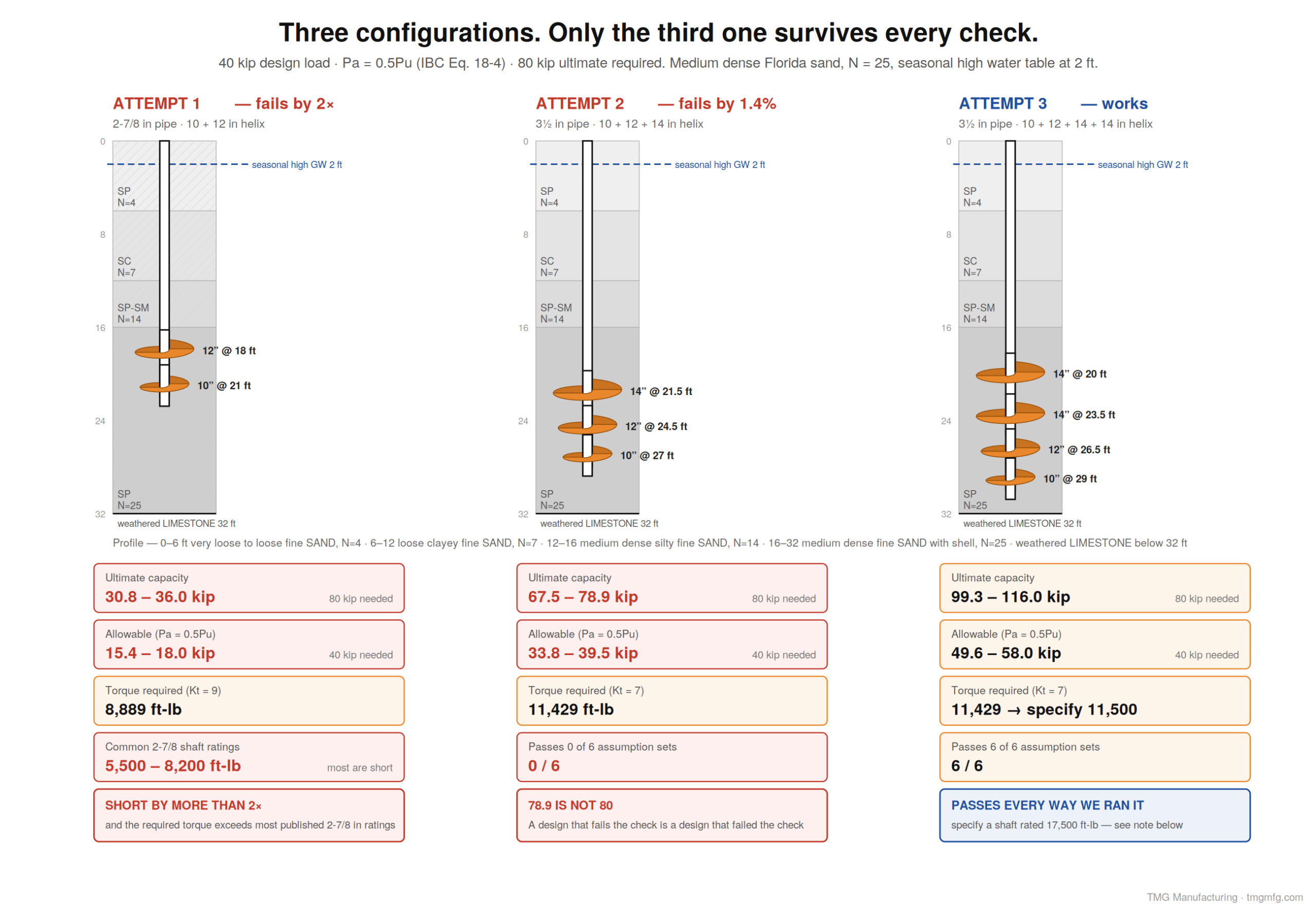
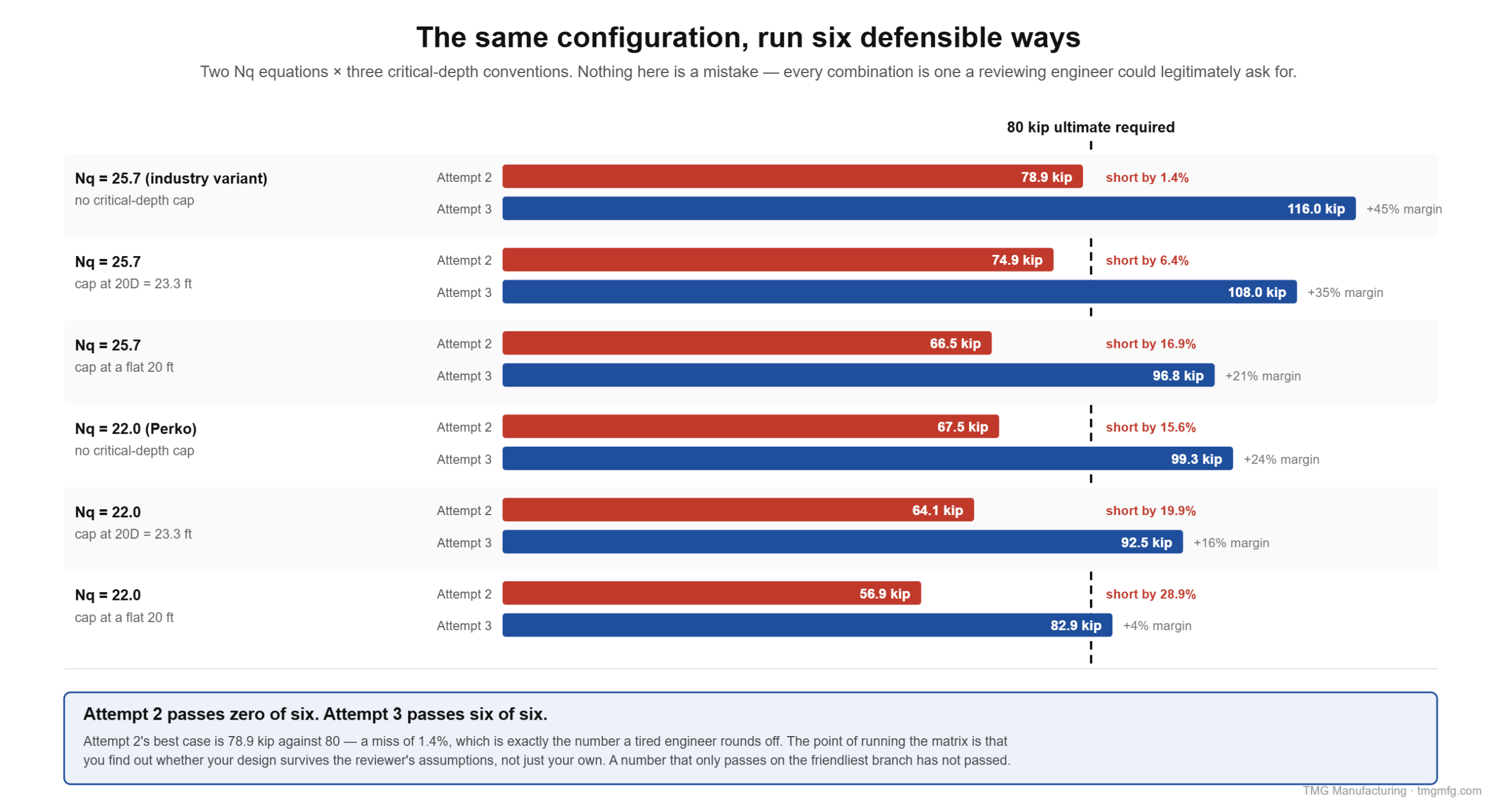
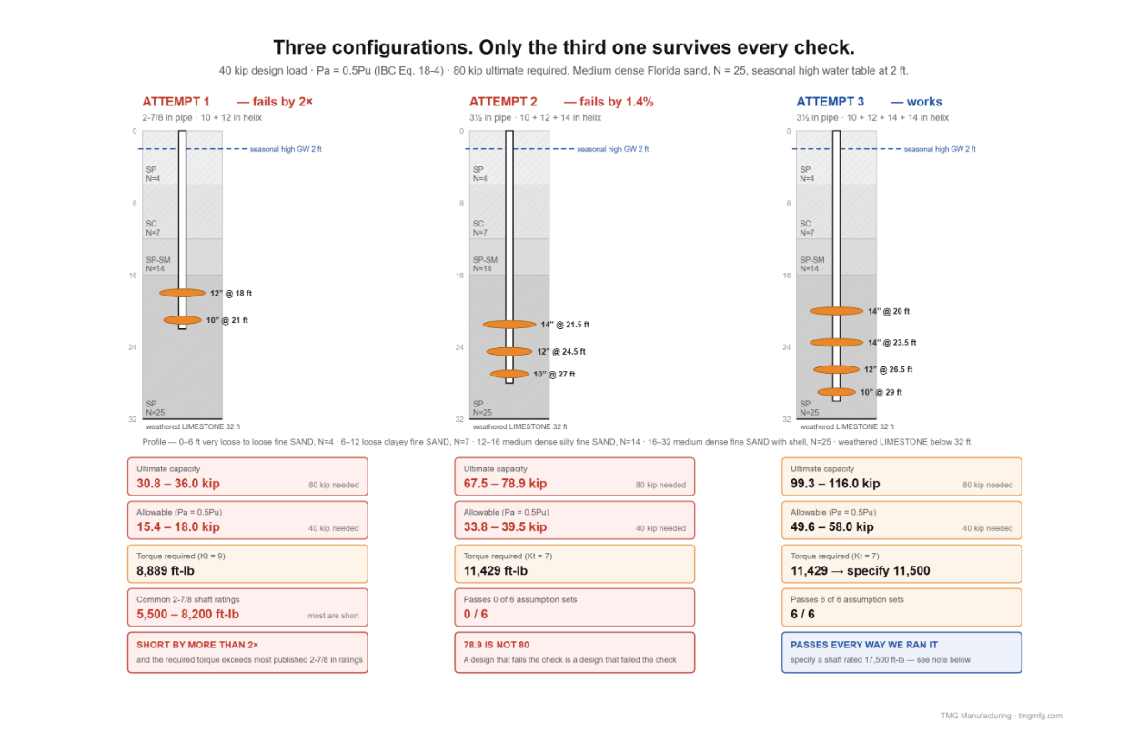
    The three configurations side by side, against the 80 kip ultimate the design load requires.
    Two Nq equations by three critical-depth conventions. Attempt two misses all six; attempt three clears all six.

    The critical-depth caveat, stated honestly

    Some offices cap effective overburden below a critical depth, on the reasoning that q’ stops increasing linearly in sand. The number matters enormously, and the commonly-repeated “20 feet” is not what the source says. The paper most often cited for it recommends 20D to 30D where D is the largest helix plate diameter, noting published values range from 10D to 40D.

    For our 14-inch plate that is 23.3 to 35 ft — meaning at 30D no cap applies to this pile at all, while the flat 20-foot cap in our table is 17D, below the low end of the recommended range. We included it anyway, as the most punitive assumption available. State which convention you used. It is judgment, not derivation, and on a marginal design it decides the answer.

    Writing the acceptance criterion

    The output of all this is two numbers on a drawing:

    Install to a minimum effective installation torque of 11,500 ft-lb, measured as the average over the final 3 feet of advance, and to a minimum lead-helix depth of 29 ft below existing grade.

    Both conditions, not either. Torque alone is not enough — a pile can hit design torque in a two-foot dense crust at 8 ft and be nowhere near the bearing stratum. Depth alone is not enough either, because the stratum moves between borings.

    Note the wording: lead-helix depth, not tip elevation. The lead helix on a manufactured lead section sits a few inches above the tip, so a “tip at 29 ft” instruction puts your bearing plate shallower than you designed it. And if you do write an elevation, name the datum.

    Where this goes wrong

    Each of these has a direction. Knowing which errors are safe and which are dangerous matters more than knowing the list.

    Forgetting buoyancy — dangerous. Using total instead of effective unit weight below the water table in this profile takes q'(18) from 1,058 to 2,056 psf, nearly double, and Attempt one’s Qult from 36.0 to 70.3 kip. A 95% overestimate, in the direction that gets a foundation built on air.

    Designing to the measured water table instead of the seasonal high — dangerous. In this profile it is about 7%. In a flatter one it is more.

    Using uncorrected N-values — direction depends on the hammer. On an automatic hammer, raw N under-predicts and you leave capacity on the table — costly, not unsafe. On a safety hammer the correction runs the other way, and treating raw N as N60 is unconservative. Find the energy ratio before you decide which mistake you are making.

    Feeding N60 into a correlation written for (N1)60 — conservative here, but wrong. Hatanaka & Uchida on N60 instead of (N1)60 gives about 42° instead of 47° in this profile. Safe direction, still an error, and it will be caught.

    A bearing layer that’s too thin — dangerous. If a helix sits an inch above a change from dense to soft and you only compute at that elevation, the answer is derived entirely from the dense layer. Compute at the helix depth and one and two diameters below, and take the lowest. In Florida this bites specifically at the sand-over-weathered-limestone contact — where, as Tampa B-01 shows, “soft clayey weathered limestone, N=12” can be weaker than the sand above it.

    Ignoring the shaft’s torque rating — dangerous in the field, not on paper. It does not make the pile weaker; it makes the pile stop short, which is worse because it happens at 4 p.m. with a crew standing around.

    Skipping the buckling check — dangerous. With 6 to 12 ft of N = 4 to 7 over the bearing layer, this profile is exactly the case that needs one.

    Designing below the boring — dangerous. Those Tampa borings stopped at 20 to 24 ft. Anything specified deeper is extrapolation, and our Attempt three at 29 ft would need a deeper boring than two of those three.

    Trusting one boring — dangerous. See the three-boring table above.

    What the log will not tell you

    Corrosion parameters. A standard geotechnical boring log for a building foundation contains none of the electrochemical data a helical design needs: resistivity, pH, sulfates, chlorides, organic content. Those are separate tests that have to be requested — and on a coastal Florida site they are not optional.

    Note also that thresholds disagree. AC358’s scope exclusions (§1.2.2) sit at resistivity below 1,000 ohm-cm, pH below 5.5, and sulfates above 1,000 ppm. The FHWA and AASHTO “non-aggressive” criteria are far stricter — 3,000 ohm-cm and 200 ppm. AC358’s numbers are a scope exclusion, not a design criterion, and citing them as though they were a pass mark is a common error.

    Also absent: the hammer energy ratio, which moves φ by 5° or more. The seasonal high water table, often only estimated. The extent of any karst — SPT gives you circulation loss and weight-of-rod zones as indicators, not geometry. Whether the surficial soil is fill, and how old. And lateral variability, which is the whole point of the three-boring table.


    Want a second set of eyes on a configuration? TMG manufactures helical piles, pile caps, brackets, and underpinning products in Tampa, and builds the SPT and CPT rigs that produce the logs behind them. Our Helical Pier Load Calculator is a quick way to check a configuration before it reaches a drawing. Call (813) 464-2299, toll-free 1-888-508-RIGS, or email info@tmgmfg.com.

    Ramzy Moumneh, TMG Manufacturing — Tampa, Florida. TMG builds geotechnical drill rigs and deep foundation products.


    FAQ

    How do you size a helical pile from a boring log? Pick a bearing stratum with adequate N-value and thickness, compute effective overburden stress at each proposed helix depth using buoyant unit weights below the seasonal high water table, convert corrected N to a friction angle, and sum Ah(c·Nc + q’·Nq) across the plates. IBC Equation 18-4 then sets the allowable load at half that ultimate.

    What N-value do you need for a helical pile bearing stratum? There is no code number. AC358 defines firm soil as N ≥ 5, which is a lateral-support threshold rather than a bearing criterion. Practical judgment puts a usable bearing layer at N ≥ 10 to 15 in sand and 8 to 10 in clay, with at least three helix diameters of that material below the lead plate.

    Do you use raw N-values or corrected ones for helical pile design? Corrected. Published correlations are written for N60. The correction can go either way — an automatic hammer pushes N up by about a third, a safety hammer pulls it down — and because Nq is exponential in friction angle, either error moves computed capacity substantially.

    How do you calculate the installation torque to specify? Divide the required ultimate capacity by the shaft’s Kt factor. AC358 §3.13.1.1 gives Kt = 9 ft⁻¹ for 2⅞-inch round shafts and 7 ft⁻¹ for 3½-inch, so 80 kip ultimate on a 3½-inch shaft requires about 11,400 ft-lb. Then check that number against the shaft’s published torsional rating — and against the torque the soil will actually generate at your design depth, which is usually higher.

    Why does the water table matter so much for helical piles in Florida? Helix bearing capacity in sand is directly proportional to effective overburden stress. Below the water table, buoyancy roughly halves the effective unit weight. In a typical Tampa profile, using total stress instead of effective inflates computed capacity by about 95%.


    Sources

    • IBC §1810.3.3.1.9 and Equation 18-4 (allowable axial load of helical piles); adopted in Florida through the FBC deep-foundation provisions
    • ICC-ES AC358, Acceptance Criteria for Helical Pile Systems and Devices — §1.2.2 (corrosion scope), §3.11.2.1 (soil definitions), §3.13.1.1 (Kt values), §4.4.1.1 and §6.9 (tension embedment), §6.7 (pile-to-pile spacing), Table 3 (helix spacing conformance window for default Kt)
    • ICC-ES evaluation reports ESR-1854, ESR-3074, ESR-3418 and ESR-3982, and current manufacturer data sheets, for the published shaft torque ratings
    • Perko, Helical Piles: A Practical Guide to Design and Installation (Wiley, 2009) — Nq = 0.5(12φ)^(φ/54), after Meyerhof (1976)
    • Published industry technical literature on bearing capacity factors for helical pile design (Nq = 1 + 0.56(12φ)^(φ/54)) and on critical depth in sands (20D–30D of the largest plate)
    • DFI Helical Pile Foundation Design Guide, 1st Edition (2019)
    • Peck, Hanson & Thornburn (Wolff 1989 fit); Kulhawy & Mayne (1990); Hatanaka & Uchida (1996)
    • Reid, A. and Taylor, J., “The misuse of SPTs in fine soils and the implications of Eurocode 7,” Ground Engineering, July 2010
    • City of Tampa 30th Street Outfall and Spring Lake Stormsewer geotechnical reports; SWFWMD geotechnical report; FDOT District 7 SR-60 geotechnical memo and Central Florida Sinkhole Evaluation
  • Wireline Core Drilling: How the System Actually Works

    Wireline Core Drilling: How the System Actually Works

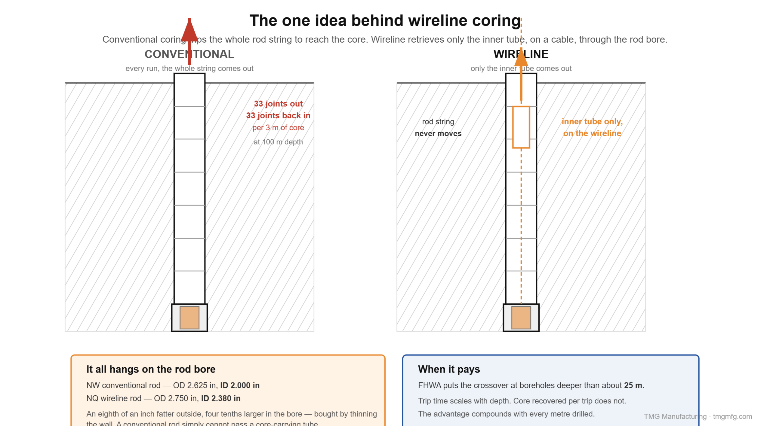
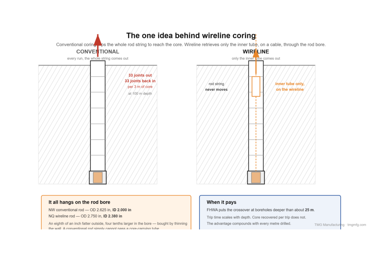
    Wireline coring retrieves the core sample without pulling the drill string. The inner tube sits inside the rotating outer barrel on a bearing, holding still while the bit cuts. At the end of a run, an overshot drops down the rod bore on a cable, latches the inner tube, and winches it out. The rods never move.

    That is the entire innovation. The system was patented in the early 1950s and in commercial use by the late 1950s. Everything else — the latch mechanism, the shut-off valves, the size designations — exists to make that one idea work reliably a thousand feet down.

    We build SPT and coring rigs and supply wireline systems, so this is written from the equipment side: what each part does, what it sounds like when it goes wrong, and where the industry’s standards currently have a hole in them.

    The problem wireline solves

    In conventional coring, the core barrel is fixed to the bottom of the rod string. To get the core, you trip the whole string — rod by rod — then run it all back in. Trip time scales with depth. Core recovered per trip does not.

    At 100 meters with 3-meter rods, that is 33 joints broken out and 33 remade to recover 3 meters of core. At a brisk 30 seconds per joint each way, roughly 33 minutes of pure rod handling. At 200 meters it is 66 minutes. (That arithmetic is ours, not a published figure.)

    In wireline coring, only the inner tube comes up. FHWA puts the crossover where wireline becomes economical at boreholes deeper than about 25 meters.

    The whole design hangs on one dimension:

    Rod Outside diameter Inside diameter
    NW (conventional) 2.625 in 2.000 in
    NQ (wireline) 2.750 in 2.380 in

    The NQ rod is an eighth of an inch fatter outside but nearly four tenths larger in the bore, bought by thinning the wall. That bore is what an inner tube and an overshot have to pass through. A conventional NW rod cannot pass a core-carrying tube — which is why “enlarged inside diameter” is in the definition of the method.

    Wireline coring retrieves the core without pulling the drill string — the inner tube comes up the rod bore on a cable.

    The cycle, step by step

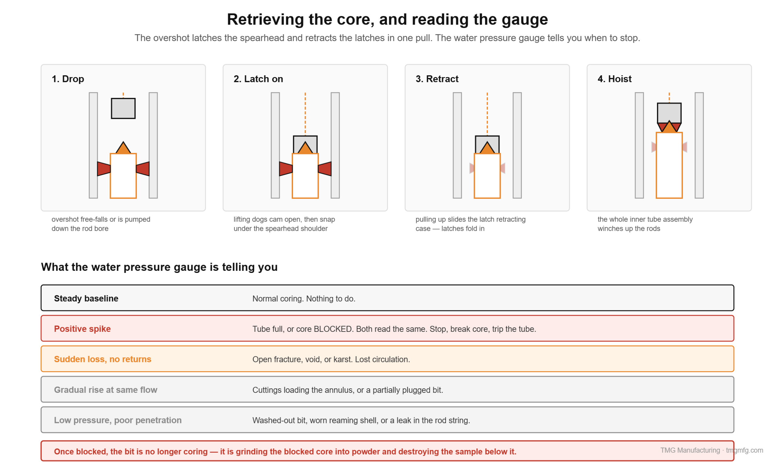
    1. Drill the run. The outer assembly rotates. The inner tube sits latched inside it, not rotating. Core enters the inner tube as the bit advances.
    2. Detect the end of run. Either the run length is reached, or the tube fills or blocks — signalled by a pressure spike on the surface water gauge.
    3. Break the core. Lift the string slightly. The core lifter is dragged up into the taper of its case, wedging onto the core and snapping it off.
    4. Trip the inner tube. Break off the water swivel and drop the overshot on the wireline cable — free-fall in a shallow hole, pumped in on a deep or angled one.
    5. Latch on. The overshot’s spring-loaded lifting dogs snap over the spearhead point.
    6. Retract the latches. Pulling up slides the latch retracting case, camming the latches inward and out of the locking coupling.
    7. Hoist the inner tube assembly up the rod bore.
    8. Empty and re-run. Drop the empty tube back down, it lands on the landing ring, the latches spring back out, and the next run starts.
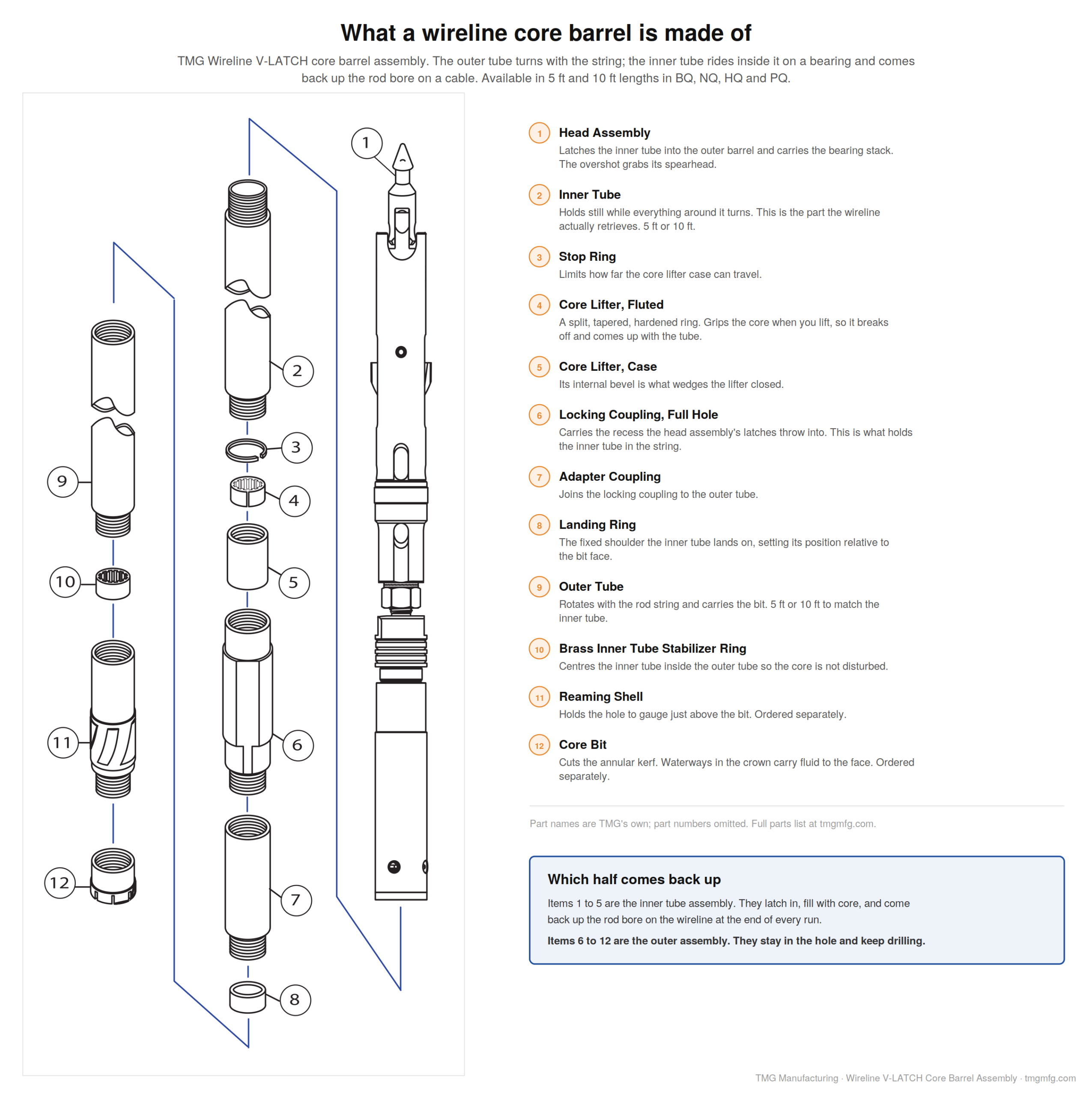
    A TMG Wireline V-LATCH core barrel, exploded. Items 1 to 5 come back up the rod bore on the wireline; items 6 to 12 stay in the hole and keep drilling.

    Anatomy: the outer assembly

    Everything here rotates.

    Component What it does
    Core bit Cuts the annular kerf. Waterways in the crown carry fluid to the face.
    Reaming shell Sits behind the bit, diamond- or carbide-set on the outside. Maintains hole gauge so the bit isn’t the only thing holding size, and stabilizes it. A worn reaming shell means an undersized hole and eventually a stuck string.
    Outer tube The rotating body. Standard 5 or 10 ft.
    Locking coupling Threaded in above the outer tube, machined with an internal recess — this is the seat the latches engage.
    Landing ring Fixed shoulder inside the outer tube. The inner tube lands on it, setting its position relative to the bit.

    Anatomy: the inner tube and head assembly

    This is the part most explanations skip. Manufacturers stack these in slightly different orders, so treat it as the parts list rather than a strict top-to-bottom section:

    1. Spearhead point — hardened and pointed, the feature the overshot grabs. It pivots, so the assembly can be swung 90° coming out of the mast.
    2. Latch retracting case — the sleeve over the latch mechanism. Pulling up on the spearhead slides it and retracts the latches. This is the release.
    3. Latches — spring-loaded arms that throw outward into the locking coupling’s recess. Original pivoting latches were 5/16 in thick; later designs doubled that, and current roller-type latches trade pivots for self-locking rollers.
    4. Landing indicator bushing and ball — a ball seated in a nylon bushing. As the tube lands and the string fills with water, pressure builds until the ball is forced through the bushing. That spike on the surface gauge is the driller’s confirmation that the inner tube has seated and latched, before coring starts. It is a landing signal. Do not confuse it with the check valve, which is a separate one-way valve down in the inner tube’s bottom C-cap.
    5. Landing shoulder — seats on the outer tube’s landing ring, stopping downward travel.
    6. Water ports — let drilling fluid bypass the landing ring and continue down to the bit face. Without them, landing the tube would deadhead the pump.
    7. Shut-off valves — rubber or nylon discs. When core fills or jams, they compress axially, expand radially against the outer tube, and choke the bypass — producing the pressure spike that ends a run. Valve hardness is selected for the ground: softer in soft formations where core loss is the risk, harder in competent rock.
    8. Compression spring — compresses on lift-off so the core lifter case can bear on the bit and transfer the load that breaks the core.

    Then the inner tube itself, the core lifter — a split, tapered, hardened ring — and its case, whose internal bevel does the wedging.

    The bearing is the whole idea

    The outer tube turns — a few hundred rpm on the large sizes, faster on the small ones, and always faster than anything you would want a rock core subjected to. Inside it is a fragile cylinder of rock, sometimes broken into loose pieces, sometimes weathered and clay-rich.

    If the inner tube turned with it, the core would be ground and twisted apart. That is exactly why single-tube barrels are limited to massive, hard, homogeneous rock.

    The swivel-type double tube solves it with a bearing stack in the head: a spindle shaft connecting the rotating upper half to the stationary lower half, a thrust bearing taking the axial load, and a spindle bushing giving radial support.

    The consequence is worth stating plainly: the rotating outer tube never drives the core in torsion. The core is pushed straight up into a tube that isn’t turning. It still sees bending and vibration, and it still gets loaded axially when you break it off at the end of a run — but it is not being wrung.

    The maintenance implication follows directly. Grease the thrust bearing, spindle bushing and hanger bearing after each retrieval. A seized bearing turns a swivel barrel into a rigid one instantly, and the first symptom is a run of ground-up core.

    Double tube or triple tube

    Double tube Triple tube (NQ3, HQ3, PQ3)
    Construction Outer + swivel-mounted inner tube Same, plus a split liner inside the inner tube
    Core size Full for the hole Smaller — the liner costs you diameter
    Extraction Pumped or tapped out of the inner tube Split tube withdrawn and opened like a clamshell
    Use when Competent, intact rock Broken, weathered, weak, or structurally sensitive rock

    For geotechnical work this is close to a settled question. USBR’s core logging guidance is blunt: split-tube core barrels should be used. The reason is not core quality for its own sake — it is that a fracture created while ramming core out of a plain inner tube is indistinguishable from a natural one on the log, and it silently depresses RQD. If the deliverable is an accurate fracture log, triple tube is effectively mandatory in anything but massive rock.

    The cost is diameter. HQ gives 63.5 mm of core; HQ3 in the same hole gives 61.1 mm. And both NQ sizes — 47.6 mm plain, 45.1 mm for NQ3 — are already below the 54 mm generally wanted for unconfined compression specimens — worth checking before you commit to a size.

    The overshot

    A hoisting plug and cable swivel at the top, an overshot body that guides the tool over the spearhead, spring-loaded lifting dogs that snap closed beneath the spearhead’s shoulder, a dog case the operator squeezes to release, a safety pin, and on deep or angled holes a pump-in adapter so circulating fluid can push the tool down when gravity won’t.

    Worth knowing as a safety matter: the spearhead is a single point of failure carrying a core-loaded inner tube over the driller’s head, and the lifting dogs grip the spearhead rather than the tube. Inspect spearheads, and do not stand under a rising overshot. That exposure is why modern designs market so heavily around positive locking.

    The overshot: hoisting plug, cable swivel, lifting dogs, dog case and safety pin.

    Reading the water gauge

    Three signals, all on the surface pressure gauge, and knowing which is which matters:

    Tube landed — start of the run. Pressure builds as the string fills, then spikes as the landing indicator ball is forced through its nylon bushing. This one you want, and it comes before you core.

    Tube full or core blocked — end of the run, one way or the other. Here is the part most write-ups get wrong: these are not two mechanisms. A full tube and a jammed core both compress the shut-off valve discs, which expand radially against the outer tube and choke the bypass flow. Same signal, and the gauge cannot tell you which. That is exactly why the response to it is the same either way — stop, break core, and trip the tube. If you were near a full run length, it was full. If you were three feet in, it blocked.

    Once blocked, the bit is no longer coring — it is grinding the blocked core into powder and destroying the sample below it. Continuing past a block signal is the single most common cause of catastrophic recovery loss on a run. Stop, break core, trip the tube.

    One caution: the signal is only as good as the shut-off valve. Worn or wrongly specified valves give no signal at all, and you find out at surface.

    Other readings worth knowing:

    • Sudden pressure loss with lost returns — an open fracture, void, or karst.
    • Gradually rising pressure at constant flow — cuttings loading the annulus, or a partially plugged bit.
    • Low pressure with poor penetration — washed-out bit, worn reaming shell, or a leak in the rod string.

    Sizes: NQ, HQ, PQ — and the NWL question

    The letter conventions come from DCDMA. The first letter is the size family, smallest to largest: R, E, A, B, N, H, P. The second is the series — X is flush-coupled (box thread at both ends, joined by a pin-to-pin coupling, thinner wall), W is flush-jointed (integral pin and box, heavier wall). WL means wireline. Q is not a DCDMA letter at all: it is one manufacturer’s proprietary system designation from the 1950s, a brand name that became the whole industry’s vocabulary. A numeric 3 means triple tube.

    Size Core diameter Hole diameter Rod OD / ID Rod weight
    BQ 1.433 in / 36.4 mm 2.345 in / 59.6 mm 2.19 / 1.81 in ~40 lb per 10 ft
    NQ 1.875 in / 47.6 mm 2.965 in / 75.3 mm 2.75 / 2.38 in 52.4 lb per 10 ft
    NQ3 1.78 in / 45.1 mm 2.965 in / 75.3 mm — —
    HQ 2.500 in / 63.5 mm 3.763 in / 95.6 mm 3.50 / 3.06 in 76.9 lb per 10 ft
    HQ3 2.41 in / 61.1 mm 3.763 in / 95.6 mm — —
    PQ 3.345 in / 85.0 mm 4.805 in / 122.0 mm 4.50 / 4.00 in 117.0 lb per 10 ft
    PQ3 3.27 in / 83.1 mm 4.805 in / 122.0 mm — —

    Now the NWL question, because the common answer is half wrong.

    In current commercial practice, NWL is normally a synonym for NQ — distributors use the terms interchangeably in the same catalog, and most manufacturers outside that original line use the WL suffix for what are NQ dimensions.

    But NXWL is not NQ. ASTM’s own tables listed them as separate rows with different numbers: NXWL cuts a 2.000 in core, NQ cuts 1.875 in. At H size the difference is larger still — HXWL cuts 61.0 mm core in a 92.7 mm hole, HQ cuts 63.5 mm in a 96.3 mm hole. (That HQ hole figure is ASTM’s; the major manufacturer catalogs publish 95.6 mm for the same size, which is the number in our table above. Manufacturers differ by a few tenths of a millimetre, and ASTM’s own footnote says so.) Different holes entirely. Not interchangeable.

    The reason there are two vocabularies is trademark and lineage, not engineering. One maker got there first, so Q dimensions became the de facto standard and everyone else labeled theirs WL. The safe procedure is unchanged: check the specific manufacturer’s dimension table before mixing tooling. ASTM said as much itself — wireline dimensions and designations vary by manufacturer.

    Rod weight matters more than people expect. A 1,000 ft NQ string is roughly 5,200 lb of steel before you add the barrel; at HQ it is 7,700 lb. That is hoist capacity, mast rating, and rig weight, and it is why size selection is a rig decision as much as a geology decision.

    Water flow and pressure

    Clear water is the standard fluid for geotechnical rock coring. Mud can be used for hole stability, but it clogs open joints and fractures — which invalidates permeability testing and piezometer installation. On a mineral hole nobody minds. On a geotechnical hole that will be packer-tested, it can void the investigation.

    Published flow recommendations vary by source. A defensible range:

    Size Flow
    BQ 20–30 L/min (5–8 gpm)
    NQ 35–50 L/min (9–13 gpm)
    HQ 50–70 L/min (13–18 gpm)
    PQ 80–100 L/min (21–26 gpm)

    Here is the rule hiding under that table. Work out the annular area for each size — hole diameter minus rod diameter, and remember that on a wireline string that gap is only about an eighth of an inch on a side — then divide the recommended flow by it. The low end of every size lands within a few percent of the same uphole velocity:

    Annulus Low end High end
    BQ 0.55 in² 184 ft/min 276
    NQ 0.97 in² 184 ft/min 263
    HQ 1.50 in² 170 ft/min 237
    PQ 2.23 in² 183 ft/min 228

    You are not pumping 35 L/min because it is NQ. You are pumping whatever lifts cuttings at roughly 170 to 185 feet per minute, and the published tables are that one number translated into four rod sizes. Those velocities are high compared with what a mud rotary hand expects, and the reason is the annulus: a wireline string barely leaves room for the fluid to get past. (Annulus areas and velocities are our own arithmetic from published hole and rod dimensions.)

    Pump pressure is not a spec — it is a consequence. No standard specifies a coring pressure. It is whatever the system needs to push the target flow through the rod bore, the bit waterways, and back up the annulus at a given depth. It rises with depth, viscosity, reduced clearance, and a blocked core.

    Flow and recovery have a two-sided optimum. Too little and the bit overheats and glazes while cuttings recirculate and grind the core. Too much and the jet erodes soft, weathered, or fractured core at the face before it enters the tube — and that disproportionately destroys the weak zones that matter most geotechnically. Higher flow in soft fractured rock to clear cuttings; lower flow in hard competent rock to prevent polishing.

    Handling the core

    Run length: 3 m maximum, reduced to 1.5 m or less just below the rock surface and in highly fractured or weathered zones. Shorter runs in bad ground is the cheapest recovery improvement available.

    Core goes into the box left to right, top to bottom — reading like a book. Use spacer blocks to mark run boundaries, and represent core loss physically with a spacer of equal length. Letting recovered core close the gap silently fabricates depth accuracy.

    Mark mechanical breaks so the logger can tell them from natural ones. FHWA specifies three short parallel lines across the fracture trace. USBR’s field manual asks only that a line be drawn across the core to denote a mechanical break, without prescribing a form. Neither is universal, and neither is enforceable across a project by itself — so the actual professional requirement is that the project’s logging procedure defines a convention and everyone applies it.

    Bit selection, briefly

    Surface-set, impregnated diamond, or PDC. The governing rule of thumb is inverse: soft matrix for hard rock, hard matrix for soft rock — the matrix has to erode fast enough to keep exposing fresh diamond, and abrasive soft formations wear a soft matrix away before the diamonds are used. Waterway design controls cooling and cuttings clearance at the face. We’ll give bit selection its own post.

    The standards problem nobody is talking about

    This is worth knowing before you write your next specification.

    ASTM D2113, the rock core drilling standard, was withdrawn in January 2023 with no replacement. ASTM D6032, the RQD standard, was withdrawn in 2026, also with no replacement. Reinstatement work items are open on both, but as of today:

    There is no active ASTM standard for rock core drilling, and no active ASTM standard for RQD.

    Anyone writing “core in accordance with ASTM D2113” is citing a withdrawn document. One live alternative exists for the drilling itself: AASHTO T 225, Diamond Core Drilling for Site Investigation. For field logging, ASTM D5434-25. Be careful with ASTM D6286 — it turns up on substitution lists, but it is a guide for selecting drilling methods, not a method. You cannot core to it any more than you can core to a catalog. That last one has an encouraging history: D5434 was itself withdrawn in 2021 and reinstated in 2025, which is the precedent the D2113 and D6032 reinstatement efforts are following.

    One casualty worth noting: D2113 carried a recovery threshold — stop core drilling when recovery of the solid portion equals or falls below 50%, or whatever percent recovery level is unacceptable to the project — and adjust RPM, feed pressure, fluid flow, or barrel and bit type when recovery drops below 100%. The 2014 revision deliberately softened that from an absolute rule to a project-defined one. That guidance left the active standards library when the standard was withdrawn. It is still good practice. It just no longer has a document behind it.


    Specifying a coring program or looking at rigs? TMG builds SPT and coring rigs and supplies wireline systems including large-diameter Geobor tooling — and we repair hydraulic drill rigs regardless of who built them. Call (813) 464-2299, toll-free 1-888-508-RIGS, or email info@tmgmfg.com.

    Ramzy Moumneh, TMG Manufacturing — Tampa, Florida. TMG builds geotechnical drill rigs and deep foundation products.


    FAQ

    What is wireline core drilling? A coring method where the inner tube holding the core is retrieved on a cable through the drill rod bore, using an overshot, without tripping the rod string. The rods stay in the hole; only the core comes out.

    What is the difference between NQ and NWL? In current practice they are used interchangeably — most NWL tooling is built to NQ dimensions. NXWL is a genuinely different size, cutting a 2.000-inch core against NQ’s 1.875-inch. Always check the manufacturer’s dimension table before mixing tooling.

    When should you use a triple tube core barrel? Whenever the rock is broken, weathered, weak, or structurally sensitive — and effectively always for geotechnical work where the deliverable is a fracture log. The split liner lets core be removed without sliding it along a tube, which prevents drilling-induced fractures that are indistinguishable from natural ones on the log.

    How do you know the core barrel is full? A pressure spike on the surface water gauge. Both a full tube and a blocked core compress the shut-off valve discs, which expand against the outer tube and choke the bypass flow — the same signal from either cause. (A separate, earlier spike, from the landing indicator ball passing through its nylon bushing, tells you the tube landed and latched at the start of the run.) The gauge cannot distinguish full from blocked, so the response is the same: stop, break core, trip the tube.

    Is ASTM D2113 still current? No. ASTM D2113 was withdrawn in January 2023 with no replacement, and ASTM D6032 for RQD was withdrawn in 2026. Reinstatement efforts are underway. In the meantime, AASHTO T 225 is the live alternative for the drilling and ASTM D5434-25 for field logging. ASTM D6286 is sometimes offered as a substitute but is a method-selection guide, not a drilling procedure.


    Sources

    • ASTM D2113-14, Rock Core Drilling and Sampling of Rock for Site Exploration — withdrawn January 2023, no replacement
    • ASTM D6032/D6032M-17, Determining Rock Quality Designation (RQD) — withdrawn 2026, no replacement
    • ASTM D5434-25, Field Logging of Subsurface Explorations of Soil and Rock (withdrawn 2021, reinstated 2025)
    • AASHTO T 225-16 (2020), Diamond Core Drilling for Site Investigation; ASTM D6286/D6286M-20 (selection guide, not a method)
    • FHWA, Subsurface Investigations / Drilling and Sampling of Soil and Rock
    • USBR Engineering Geology Field Manual, core logging and handling chapters
    • Manufacturer diamond-products and coring-rod catalogs; published core barrel head assembly technical documentation
    • Drilling-fluid product literature and published bit-wear guidance
  • Helical Piles: The Pros and Cons

    Helical Piles: The Pros and Cons

    Helical piles install fast, quiet, and vibration-free with small equipment, reach limited-access sites, and are the only deep foundation whose design capacity is routinely accepted from an installation-torque correlation written into code. They lose to micropiles and drilled shafts in gravel, cobbles, very dense soil, and aggressive soils.

    That summary is deliberately two-sided, because a helical pile article that only lists advantages is useless to the person who signs the drawings. Helicals are an excellent tool inside their envelope and a poor one outside it, and the boundary is sharper than most marketing suggests.

    TMG Manufacturing sits on both sides of this. We build the rigs that collect the subsurface data — SPT, coring, CPT and DMT push rigs — and we manufacture the helical piles, underpinning brackets, pin piles, drill-in piles, and micropile products designed from that data. When a boring log says a helical is the wrong answer, we are the ones selling the alternative. That is why the “cons” section is the longer one.

    How a Helical Pile Carries Load

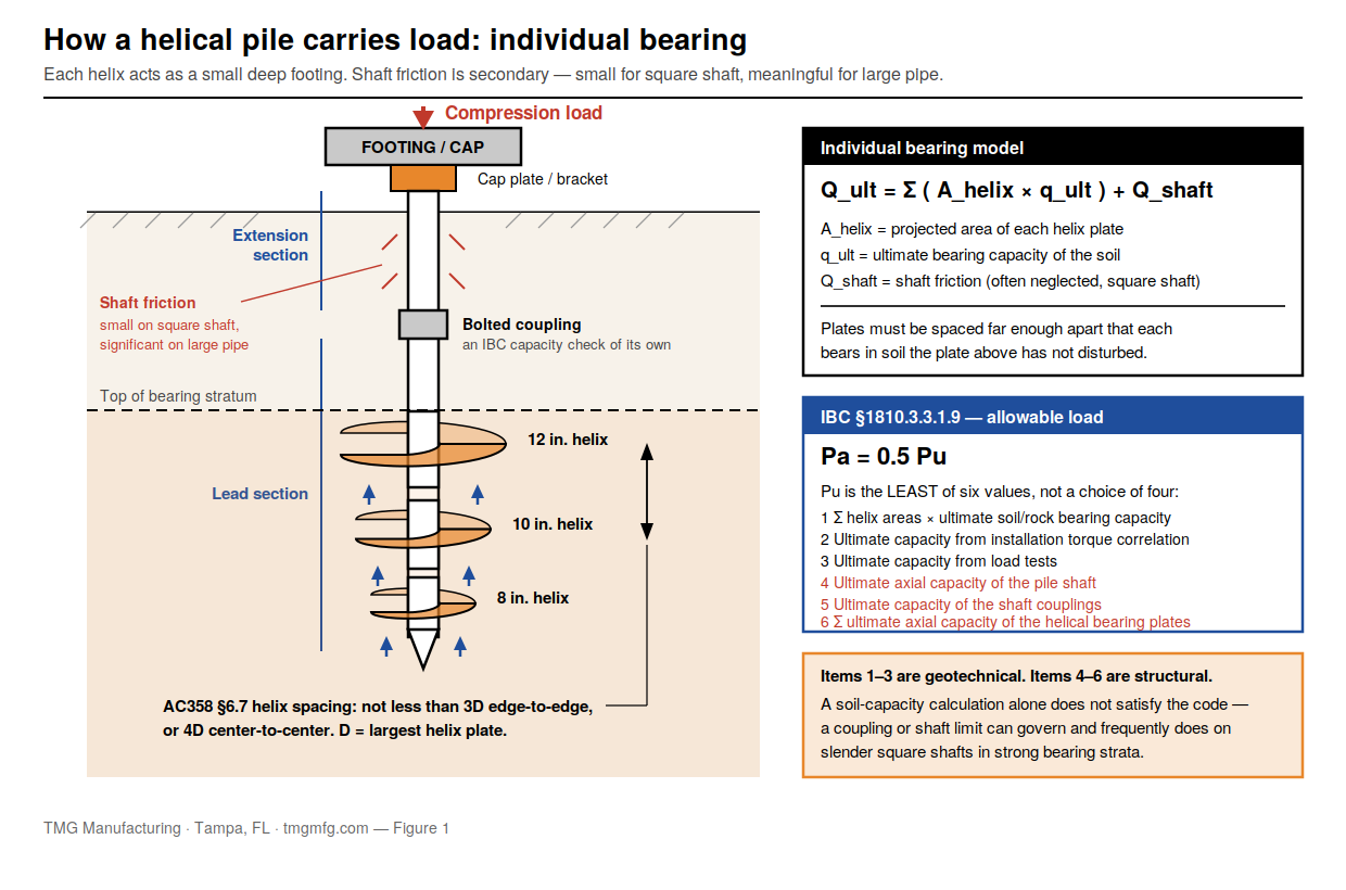
    A helical pile is a steel shaft with one or more helix-shaped bearing plates welded to it, rotated into the ground by a hydraulic torque motor. Each helix advances roughly one pitch per revolution — about 3 inches — so the pile screws in rather than displacing soil laterally the way a driven pile does.

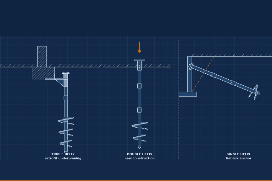
    Load transfers two ways. The dominant mechanism is individual bearing: each plate acts as a small deep footing, and geotechnical capacity is the sum of the plates’ bearing capacities. The secondary mechanism is shaft friction — small for a square shaft, meaningful for large pipe. In tension the same helices work in uplift, which is why helicals dominate the tieback and guy anchor market.

    Figure 1 — Helical pile load transfer and anatomy
    Shaft, lead section, helix plates, coupling, and the individual-bearing load transfer model.

    Configurations and Shaft Sizes

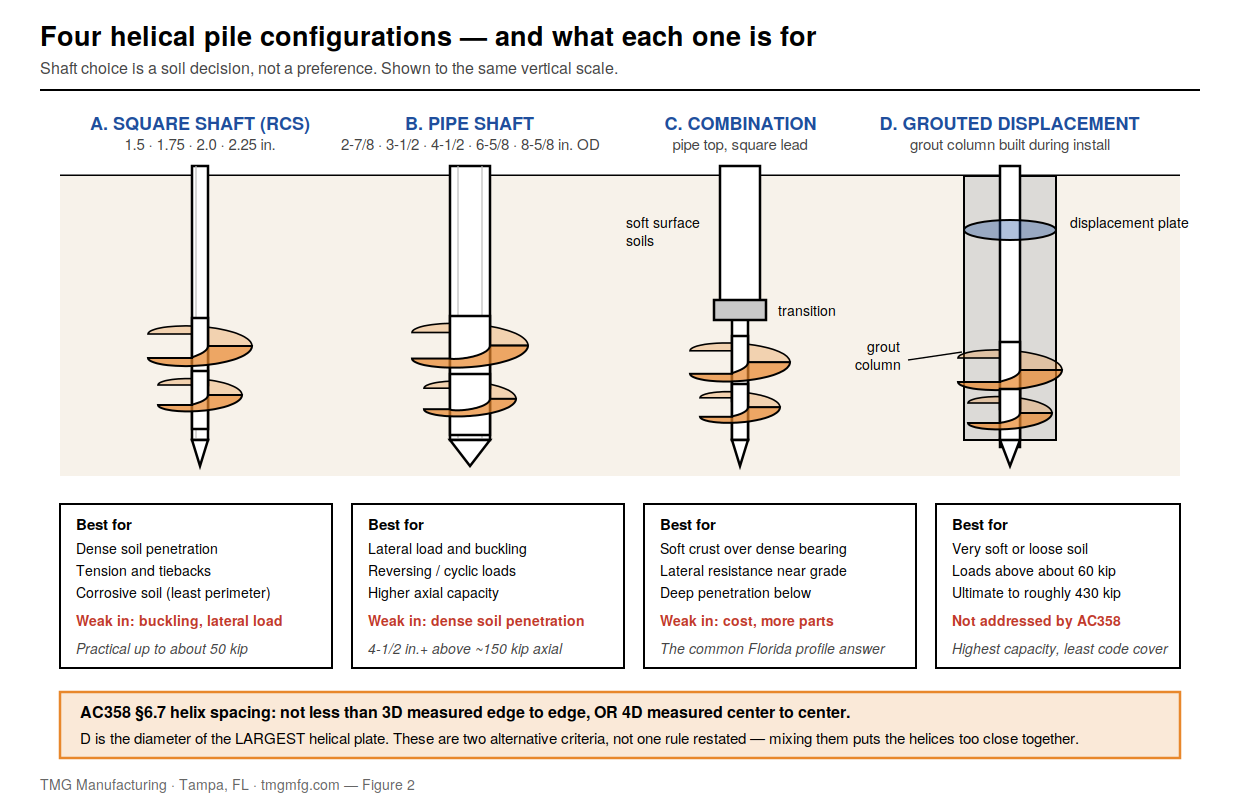
    • Square shaft (round-corner square, “RCS”). 1.5, 1.75, 2.0, and 2.25 in. Highest torque capacity per pound of steel, least soil disturbance, least perimeter exposed to corrosion, best penetration into dense soil. Weak in buckling and lateral load. Manufacturer guidance puts the practical sweet spot at working loads up to roughly 50 kips.
    • Pipe shaft. 2⅞, 3½, 4½, 6⅝, and 8⅝ in. OD. Far better lateral and buckling resistance, more shaft friction, more capacity — manufacturers recommend the 4½ in. and larger line for axial loads above about 150 kips and lateral loads above about 5 kips.
    • Combination. Pipe on top for lateral and buckling resistance, square lead for penetration. Common where soft surface soils overlie a dense bearing stratum.
    • Grouted displacement pile. A displacement plate builds a grout column around the shaft as it advances. Manufacturer literature reaches into the 400-kip ultimate range, and it is the standard answer in very soft or loose soil where an ungrouted shaft would buckle.

    Helix plates are spaced so each bears in relatively undisturbed soil. ICC-ES AC358 §6.7 states the rule as not less than 3D edge to edge, or 4D center to center, where D is the diameter of the largest helical plate. Those are two alternative criteria, not one rule restated — mixing them puts your helices too close together.

    Figure 2 — Helix configurations and spacing
    Square, pipe, combination, and displacement configurations, with the AC358 helix spacing rule.

    The Pros and Cons, Side by Side

    Factor Helical pile Honest assessment
    Installation speed Piles per hour, not per day; immediate loading Real advantage; often decides schedule-driven repairs
    Installed cost Low, in the right soil Disappears fast in dense or gravelly soil where installation stalls
    Vibration Effectively none Real advantage next to sensitive or historic structures
    Noise Hydraulic motor only; no impact Real advantage in occupied buildings and residential work
    Equipment size Mini excavator, skid steer, or handheld Often the only option in a basement or crawlspace
    Capacity verification Torque correlates to capacity Unusual among deep foundations — but conditional and size-limited
    Spoil generation None Advantage on contaminated or landfill sites
    Tension capacity Excellent Best-in-class for uplift and tiebacks
    Weather / groundwater Installs saturated; no dewatering, no curing Advantage in Florida-type conditions
    Dense sand, gravel, cobbles Poor Stalls or grinds; often a hard stop
    High-capacity loads Limited on common shaft sizes Torque verification drops out of AC358 scope on the largest shafts
    Aggressive soils Poor without design attention 50-year sacrificial basis; excluded outright below 1,000 ohm-cm
    Buckling in very soft soil Poor for slender shafts Below about N = 4, buckling governs, not bearing
    Public design guidance Thin No dedicated FHWA manual, no dedicated AASHTO LRFD section

    Torque Correlation: The Advantage Nobody Else Has

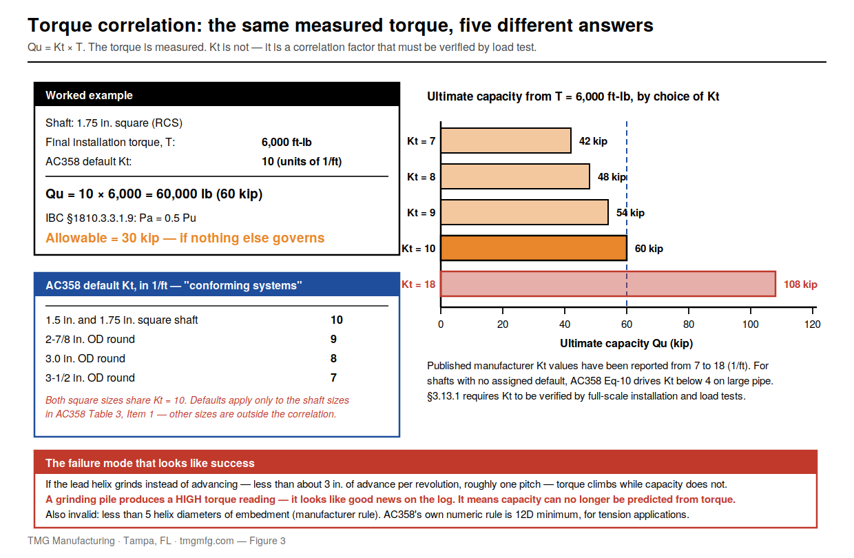
    Rotate a helical pile into the ground and the torque required to keep it turning is measured continuously by the installing equipment. That torque correlates to capacity:

    Qu = Kt × T

    where Qu is ultimate capacity, T is final installation torque, and Kt is a torque correlation factor in ft⁻¹. AC358 publishes defaults for “conforming systems”: 10 ft⁻¹ for both 1.5 in. and 1.75 in. square shaft, 9 ft⁻¹ for 2⅞ in. round, 8 ft⁻¹ for 3.0 in. round, 7 ft⁻¹ for 3½ in. round.

    Very few deep foundations give you this. A drilled shaft gives you an integrity test, not a capacity, until you load-test it. Driven piles give dynamic formulas and PDA. A helical tells you at every location whether it reached the torque the design assumed — before the structure goes on it.

    Figure 3 — Torque correlation, worked, with the Kt spread
    Worked capacity from installation torque, and how the choice of Kt changes the answer.

    The Part Nobody Tells You: When Torque Correlation Lies

    The defaults are not universal, and it is not “just use 10.” AC358 §3.13.1 requires Kt to be verified by full-scale field installation and load tests, and the published defaults still carry a verification testing schedule. They attach to specific shaft sizes only. For sizes without an assigned default, AC358 gives Kt = 22.285 (d_eff)^−0.9195, which drives Kt down sharply as the shaft grows — around 8.5 for a 2.0 in. square shaft and below 4 for large-diameter pipe. And the criteria are explicit that the correlation “applies only to shaft sizes described in Item 1 of Table 3. For shaft sizes that are outside of this prescribed range, this torque correlation is outside the scope of this criteria.” The high-capacity pipe configurations people reach for on big projects are precisely the ones where the torque-verification advantage loses its ICC-ES standing. No brochure says that.

    It inverts when the helix grinds. If the lead helix hits a hard layer and advances substantially less than its pitch — under about 3 inches per revolution — torque climbs while capacity does not. Published guidance is blunt: grinding does not mean the pile will not carry its rated load; it means capacity can no longer be predicted from torque. This is the failure mode that matters most, because it produces a high torque reading, which looks like good news on the log.

    It is invalid at shallow embedment. Manufacturer guidance requires the uppermost helix at least 5 helix diameters below grade in cohesive and fine granular soils. That 5D rule is a manufacturer rule, not code and not AC358 — AC358’s own numeric rule is 12D for tension applications, with anything shallower requiring a registered design professional to set the depth.

    It is calibrated on clay. Kt = 10 performs well in cohesive soils and tends to be conservative in clean granular soils. In sand it may leave capacity on the table; in a soil the correlation was never calibrated for, it may do the opposite.

    One citation warning. A frequently referenced ASCE Journal of Performance of Constructed Facilities paper on installation torque and axial capacity in cohesionless soils has been retracted by ASCE, and is still cited widely without any retraction notice. If a design basis on your desk rests on it, check the source.

    What the Code Actually Requires

    IBC §1810.3.3.1.9 governs helical pile allowable capacity, with the same section number in the 2021 and 2024 IBC. It is routinely described online as “four methods.” It is not. It sets Pa = 0.5 Pu (Equation 18-4), where Pu is the least of six values: (1) sum of helix plate areas × ultimate soil or rock bearing capacity; (2) ultimate capacity from well-documented correlations with installation torque; (3) ultimate capacity from load tests; (4) ultimate axial capacity of the pile shaft; (5) ultimate capacity of the shaft couplings; (6) sum of the ultimate axial capacity of the helical bearing plates. Items 1–3 are geotechnical, 4–6 structural, and 0.5 is a blanket factor of safety of 2 on whichever governs.

    IBC §1810.3.1.5, the design-conditions provision for helical piles, is one sentence and imposes no helix geometry: helical piles “shall be designed and manufactured in accordance with accepted engineering practice to resist all stresses induced by installation into the ground and service loads.” Note the second half — installation stresses are a code requirement, not an afterthought. Helix spacing and geometry rules come from AC358 or a manufacturer, not from that section.

    IBC §1810.4.11 requires a registered design professional to set embedment depth and torsional resistance criteria, and prohibits exceeding the pile’s maximum allowable installation torque. IBC §1705.9 requires continuous special inspection during installation — equipment, pile dimensions, tip elevations, final depth, final torque. It is a standalone section, not a row in a Table 1705 matrix, and was §1704.10 in the 2009 IBC.

    AC358 (24), published April 2025, is the current acceptance criteria as of August 2026. It covers axial compression, axial tension, and lateral loads, and permits Seismic Design Categories D through F where §3.14 is satisfied — older evaluation reports limiting use to SDC A, B and C are still circulating, so check the specific ESR.

    Florida. The Florida Building Code, 8th Edition (2023), based on the 2021 IBC, took effect December 31, 2023; the 9th Edition (2026) is scheduled for December 31, 2026. Florida adopts IBC Chapter 18 with state amendments, and Chapter 18 carries a separate High-Velocity Hurricane Zone block for Miami-Dade and Broward with its own pile load test provisions. Do not assume the model IBC text governs on a Florida project — check §1810 and the HVHZ sections against the FBC itself.

    Two things an evaluation report does not do: it is explicitly not an endorsement, carries no warranty, and still requires project-specific calculations and drawings by a registered design professional. “ICC approved” is not a design.

    Where Helical Piles Are the Wrong Choice

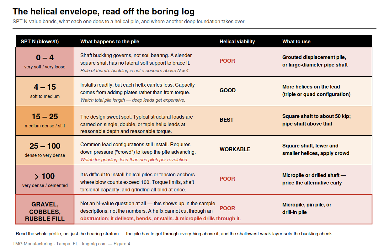
    Figure 4 — Soil profile decision guide
    N-value bands, the practical helical envelope, and where micropiles or drilled shafts take over.

    Dense and gravelly soils. Pack’s Practical Design and Inspection Guide for Helical Piles and Helical Tension Anchors puts routine installation at SPT N up to about 100 and says plainly that it is difficult above N = 100. Cobbles, boulders, and construction debris are worse than dense sand: a helix cannot cut an obstruction — it deflects, bends, or stalls. A micropile drills through what stops a helix.

    Very soft soils, for slender shafts. Manufacturer guidance treats buckling as not a concern where SPT N exceeds about 4 along the full shaft. Below that, shaft buckling — not soil bearing — governs, and you need larger pipe or a grouted displacement pile.

    High-capacity loads on common shaft sizes. Manufacturer-published ultimate capacities for solid square shafts run about 70 kips at 1.5 in., 100 at 1.75 in., 150 at 2.0 in., and 200 at 2.25 in.; allowable design load is half the governing ultimate per Equation 18-4. Large pipe and grouted displacement piles go higher, into the 400-kip range in manufacturer literature — but AC358 provides no design or acceptance provisions for grouted-shaft or displacement-plate piles, and the torque correlation drops out of scope on the largest shafts. The highest-capacity products in this category have the thinnest acceptance-criteria coverage.

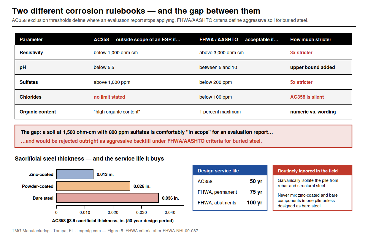
    Aggressive soils. AC358 puts helical piles outside the scope of an evaluation report where resistivity is below 1,000 ohm-cm, pH is below 5.5, sulfates exceed 1,000 ppm, or the soil has high organic content, is landfill, or is mine waste. AC358 sets no chloride limit — anyone quoting one is quoting something else.

    Compare that to the FHWA/AASHTO electrochemical criteria for steel soil reinforcement in MSE walls (FHWA-NHI-09-087): resistivity above 3,000 ohm-cm, pH between 5 and 10, chlorides under 100 ppm, sulfates under 200 ppm, organics under 1 percent. FHWA is roughly three times stricter on resistivity and five times on sulfates. A soil comfortably “in scope” for an ESR would be rejected outright as aggressive backfill under those criteria.

    Figure 5 — Corrosion thresholds and sacrificial steel
    AC358 exclusion thresholds vs. FHWA/AASHTO criteria, and the sacrificial thickness assumptions behind each.

    And the service life assumption is shorter than people think. AC358 §3.9 computes sacrificial thickness for a 50-year design period — 0.013 in. zinc-coated, 0.026 in. powder-coated, 0.036 in. bare steel. Read the powder-coated number carefully: the formula credits the coating with only 16 years, after which the steel corrodes as if bare. FHWA/AASHTO assume 75 years for permanent structures and 100 for abutments. An ESR-based helical pile is not designed to bridge-infrastructure service life, and nothing on the submittal says so.

    Two provisions get ignored in the field: AC358 §3.9 requires components to be galvanically isolated from reinforcing steel, structural steel, and other building metals; and evaluation reports prohibit mixing zinc-coated and bare steel components in one system unless the whole assembly is designed as bare steel. A galvanized lead with bare extensions voids the corrosion basis.

    Finally, the guidance gap. There is no dedicated FHWA design manual for helical piles and no dedicated AASHTO LRFD design section — FHWA NHI-05-039 is a micropile manual. Helical code standing rests on IBC §1810.3.3.1.9 plus proprietary evaluation reports. Compared with driven piles, drilled shafts, and micropiles, that is a real difference in how much of the design basis is independently reviewable.

    How to Actually Choose

    1. Read the N-value profile through the full design depth. Long stretches under about N = 4 mean buckling territory — go to pipe or displacement. N above 100 in the bearing stratum, or anywhere you must penetrate, means installation problems: price a micropile alternative now.
    2. Look for gravel, cobbles, rubble, and fill in the sample descriptions. These never show up as a single number. They show up in the driller’s log — one more reason the log has to be written properly.
    3. Order corrosion testing where it matters. Resistivity, pH, sulfates, chlorides, organics. It is inexpensive, and it is the difference between a 50-year foundation and a warranty claim.
    4. Set the load-test program before installation. ASTM D1143/D1143M-26 (static axial compression) and D3689/D3689M-25 (static axial tension) are current. Always cite the dual designation; the legacy standalone “D1143” is no longer current.
    5. Confirm the specific ESR, not the category. Kt values, seismic design category limits, shaft sizes inside the torque-correlation scope, and corrosion exclusions are all product-specific.

    For a first-pass estimate from torque and shaft type, our helical pier load calculator will get you in the right range before you commit to a configuration.


    Working through a helical pile decision? TMG Manufacturing manufactures helical piles, underpinning and foundation repair products, pin piles, drill-in piles, and compaction grouting products — and we build the SPT, CPT, and coring rigs that produce the data you need to size them. If the answer is a micropile, we will tell you. Call (813) 464-2299 or toll-free 1-888-508-RIGS, or email info@tmgmfg.com.

    Ramzy Moumneh, TMG Manufacturing

    Frequently Asked Questions

    What are the disadvantages of helical piles?

    Difficult or impossible installation in dense soil, gravel, cobbles, and rubble fill; corrosion vulnerability in aggressive soils, with evaluation reports excluding soils below 1,000 ohm-cm resistivity, below pH 5.5, or above 1,000 ppm sulfates; buckling risk in very soft soil below about SPT N = 4; a torque correlation that becomes invalid when the helix grinds, and that AC358 limits to a defined range of shaft sizes; and thinner public design guidance than micropiles or drilled shafts.

    How long do helical piles last?

    AC358 computes sacrificial steel thickness on a 50-year design period, so an evaluation-report-based helical pile is nominally a 50-year foundation in non-aggressive soil. With galvanizing and adequate shaft thickness it can last considerably longer, but that is a project-specific corrosion analysis, not a default. FHWA/AASHTO use 75 to 100 years for buried steel reinforcement in permanent structures.

    Do helical piles need a load test?

    Often not, subject to the authority having jurisdiction. IBC §1810.3.3.1.9 allows ultimate capacity to be established from well-documented correlations with installation torque, which is why torque verification substitutes for load testing on many projects. But AC358 requires Kt itself to have been verified by full-scale load tests, some jurisdictions require testing regardless, and a load test is the right call on unusual soils, high-capacity piles, shaft sizes outside the AC358 range, or any site where the helix grinds.

    How much weight can a helical pile hold?

    Manufacturer-published ultimate capacities run roughly 70 kips for a 1.5 in. square shaft, 100 kips at 1.75 in., 150 kips at 2.0 in., and 200 kips at 2.25 in.; large pipe and grouted displacement piles reach into the 400-kip range in manufacturer literature. Allowable design load is half the governing ultimate per Equation 18-4 — so a 200-kip ultimate is a 100-kip allowable at best, often less once shaft, couplings, and helix plates are checked.

    Are helical piles better than push piers?

    They solve different problems. Helical piles are torqued to a target and verified from torque without any structural reaction, so they work on new construction, light structures, and in tension. Push piers are hydraulically driven using the building’s own weight as reaction, so they need a heavy enough structure — and give you a structural load test as a byproduct. On a light residential structure, push piers may not have enough reaction to reach competent bearing; on a heavy structure over deep soft soil, they often will.


  • How to Perform SPT Testing: A Complete Field Procedure Guide

    How to Perform SPT Testing: A Complete Field Procedure Guide

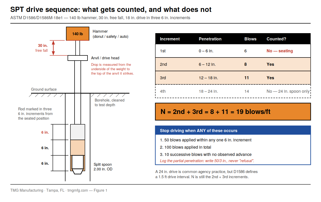
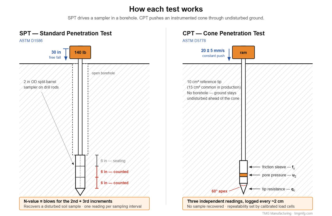
    SPT testing drives a 2-inch split-spoon sampler 18 inches into the bottom of a borehole using a 140-pound hammer falling 30 inches. Mark the rod every 6 inches, count blows for each increment, and add the second and third counts. That sum is the N-value. The first 6 inches is seating and is never counted.

    That is the whole test, and almost every part of it can be done wrong without anyone noticing. The N-value on a boring log looks like a measurement. It is really the output of a procedure — rod marking, hammer release, sampler condition, how you reached depth — and the procedure is where the error lives. A crew that seats the spoon in slough, or lets the rope drag on the cathead, hands the engineer a number that is 30 percent off and looks completely normal on the log.

    TMG Manufacturing builds the rigs that run this test and also manufactures the deep foundation products engineers design from those N-values — the hammers, tripods, split spoons and baskets, and the helical piles sized off the resulting log. We have no interest in making SPT sound more precise than it is.

    What the Standard Penetration Test Actually Measures

    The SPT measures the resistance of soil to being displaced by a driven, thick-walled tube. It is a disturbance test, not a strength test: no stress-strain curve, no undrained shear strength, no friction angle directly. Those come from correlations, and every correlation carries the scatter of the field procedure inside it.

    Governing standard: ASTM D1586/D1586M-18e1, active as of August 2026, with a revision work item (WK99626) open in subcommittee D18.02. The energy input is a 140 lb hammer falling 30 in. The current edition lists 750 mm as the separate hard-metric drop value; older editions and the ISO family use 760 mm, which is why you see both numbers in the wild.

    SPT drive sequence and N-value computation
    Figure 1. The 18-inch drive, the three 6-inch increments, and why the seating increment is discarded.

    Anatomy of a Split-Spoon Sampler

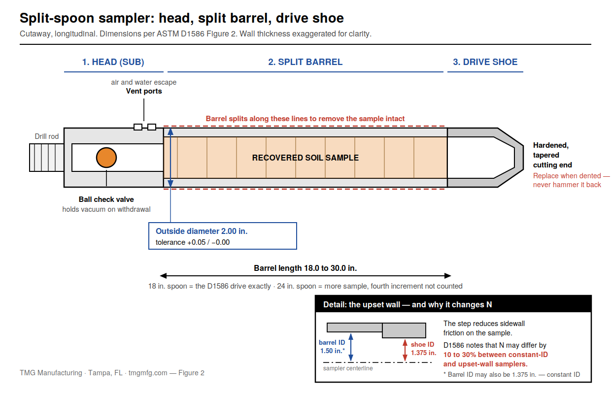
    • Head (or sub). Threads onto the drill rod. Holds the ball check valve and vent ports that let water and air escape as soil enters, and hold vacuum on withdrawal so the sample does not drop out.
    • Split barrel. Two half-cylinders clamped between head and shoe. Splitting them open is how the sample comes out intact.
    • Drive shoe. The hardened, tapered cutting end — the wear part, and the part that decides what actually gets sampled.

    Per ASTM D1586 Figure 2, the sampler is 2.00 in. OD (+0.05 / −0.00) with a drive shoe ID of 1.375 in. ± 0.005 in. The split barrel’s inside diameter may be either 1.50 in. — the “upset wall” configuration, barrel bore larger than the shoe — or 1.375 in., a constant inside diameter. Both are permitted; the upset wall reduces sidewall friction on the sample and the constant ID does not.

    That choice is not cosmetic. The standard itself notes N-values may differ by 10 to 30 percent between a constant-ID sampler and an upset-wall sampler. A 16-gauge liner in a 1.50 in. barrel is a second route to constant ID; liners are permitted, but note them on the penetration record. D1586 points to Practice D6066 for the correction — and D6066 was withdrawn in 2020, so the correction reference is a dead document.

    Barrel length is allowed to be 18.0 to 30.0 in., which is where the 18-inch versus 24-inch question comes from.

    Split-spoon sampler cutaway showing head, split barrel, and drive shoe
    Figure 2. Head, split barrel, and drive shoe, with the ASTM dimensions that define the test.

    The Field Procedure, Step by Step

    1. Advance the hole to test depth by one of the three methods below, and stop cleanly.
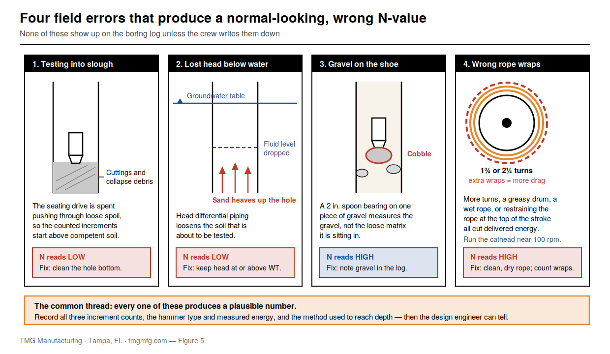
    2. Clean the bottom of the hole. Anything left in the auger shoe gets driven ahead of the spoon.
    3. Maintain hole stability. Keep water or drilling fluid at or above the groundwater table. Lost head lets the bottom heave, and heaved sand reads artificially low.
    4. Inspect and assemble the sampler. Check the shoe for dents, out-of-round, or a curled lip. Replace it — do not hammer it back. A deformed shoe changes the effective ID and the N-value with it.
    5. Lower the sampler to the bottom and set the weight of rods and hammer on it. If it sinks under its own weight, that is data — log it.
    6. Mark the drill rod in three 6-inch increments, measured up from the actual seated position, not from a nominal depth. Tape, soapstone, or a carpenter’s pencil against the rod, referenced to the drive head or rig table.
    7. Drive with the 140 lb hammer falling 30 in. Rope and cathead: 1¾ or 2¼ rope turns, cathead at a minimum of about 100 rpm, rope clean and dry, drum free of rust and grease, and no restraining the rope at the top of the stroke.
    8. Count and record blows separately for each 6-inch increment. Three numbers, always — 6/8/11, not just the sum.
    9. Compute N as the second plus third increments. Above, N = 19. The first increment is the seating drive.
    10. Stop driving if any of these occurs: 50 blows within any one 6-inch increment; 100 blows total; or 10 successive blows with no observed advance.
    11. Record partial penetration properly. Fifty blows for 3 inches is logged 50/3″ — never “refusal” with nothing behind it. The partial number is data; “refusal” is not.
    12. Open the barrel and log the sample immediately — recovery length, stratigraphy, color, moisture, consistency or density, odor, and contacts within the sample. Describe per ASTM D2488-26; classify per ASTM D2487-17(2025) where lab data justify it.
    13. Seal and label before it leaves the drill floor. Jars for classification, sealed sleeves for moisture retention. Project, boring, sample number, depth interval, blow counts, recovery.
    14. Advance to the next test depth and repeat — typically 2.5 ft or 5 ft spacing, tightened at strata contacts and bearing elevations.

    18-Inch vs. 24-Inch Split Spoons

    Both are legitimate tools; only one is running an ASTM test.

    An 18-inch spoon matches the D1586 drive interval exactly — three increments, N from the second and third, barrel full when the drive is done. Lighter, easier to open, less prone to sample compression.

    A 24-inch spoon is driven a full 24 inches in four increments. N is still increments two and three; the fourth is recorded and never counted. You gain sample volume — more for jars, more for classification testing, a better chance of catching a contact in one drive. What you should not do is call it an SPT per D1586: the standard defines a 1.5 ft drive interval and nothing else, so a 24-inch drive is practice convention, not an ASTM-defined test. Log it as a 24-inch sampling drive and you are being accurate.

    Three Ways to Get to Depth

    Three routes to SPT test depth compared
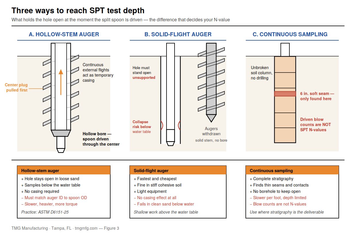
    Figure 3. Hollow-stem auger, solid-flight auger, and continuous sampling compared at the sampling interval.

    Hollow-stem auger. The flights double as temporary casing: drill to depth with a center or knock-out plug, pull the plug, sample through the hollow center. It is the default above the rock line in Florida and most of the Southeast, because the hole stays open in loose sand and you can sample below the water table without casing. Match auger ID, sampler OD, and rod OD deliberately — as trade practice, not a standards requirement, 3¼ in. and 4¼ in. ID augers are the common pairing with a 2 in. spoon. Reference practice is ASTM D6151-25 (the older D6151/D6151M-15 was withdrawn in 2024 and reinstated without the “M”).

    Solid-flight auger. No casing effect. Faster and cheaper in cohesive soils that stand open, fine above the water table. The hole must stay open unsupported while you pull augers, lower the spoon, and drive it. In clean sand below the water table it will not, and you are sampling collapse instead of soil.

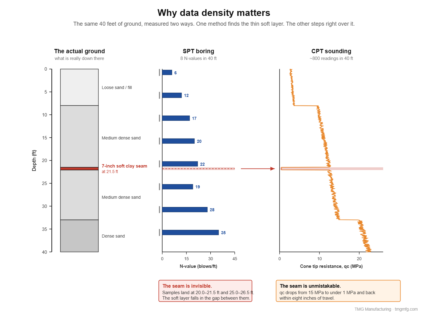
    Continuous sampling, no drilling. Drive or push a continuous sampler and recover an unbroken column of soil — complete stratigraphy instead of an 18-inch sample every 5 ft, which is the difference between finding a 6-inch soft seam and never knowing it existed. Slower per foot, depth-limited, and in a driven configuration the blow counts are not SPT N-values. Use it where stratigraphy is the deliverable.

    Mud rotary is a fourth method and deserves its own article; ASTM D5783-18(2025), which D1586 cross-references, remains active.

    The Part Nobody Tells You: Your Hammer, Not Your Soil, Sets the N-Value

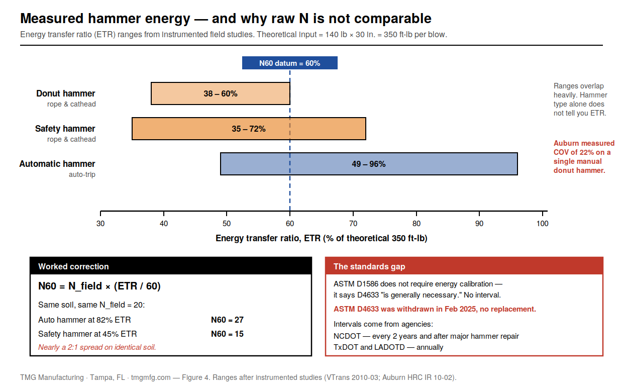
    The SPT delivers a nominal 350 ft-lb per blow (140 lb × 30 in.). Only part of that reaches the sampler, and the part that does is not constant. The fraction is the energy transfer ratio (ETR).

    Measured SPT hammer energy transfer and the N60 correction
    Figure 4. Measured ETR ranges from instrumented studies, and a worked N60 correction.

    Instrumented studies — VTrans’s hammer energy variability work and Auburn University’s Highway Research Center calibrations among them — put measured ETR at roughly 38 to 60 percent for donut hammers, 35 to 72 percent for safety hammers, and 49 to 96 percent for automatic hammers; Auburn’s calibration of six automatic hammers for ALDOT averaged about 91 percent. The widely reproduced “donut 45, safety 60, automatic 80” table is not fabricated — those are rounded averages of measured data — but the distributions behind them are wide and heavily overlapping, and Auburn measured a coefficient of variation of 22 percent on a single manual donut hammer.

    The correction: N60 = N_field × (ETR / 60). A field N of 20 from a hammer measured at 82 percent is an N60 of 27. Feed a correlation the raw 20 where 27 belongs and you are roughly 25 percent low on N — and because capacity correlations are not linear in N, the downstream error is not a simple percentage.

    Here is what catches people out. ASTM D1586 does not require energy calibration. Its scope says D4633 “is generally necessary” to measure drill rod energy — advisory language, no interval specified. And ASTM D4633 was itself withdrawn in February 2025 with no replacement, reinstatement work item open. The current SPT standard’s energy reference points at a withdrawn document.

    Intervals come from agencies instead. NCDOT requires measurement every two years and after any major hammer repair; TxDOT and LADOTD require annual calibration, and LADOTD permits automatic hammers only. A specification silent on hammer energy is silent on the largest controllable source of error in the test.

    Where SPT Does Not Work

    • Soft and sensitive clays. N near zero carries almost no information. Use thin-walled tube sampling, vane shear, or CPT.
    • Gravel, cobbles, and construction fill. A 2 in. spoon bearing on one stone gives a fake high N.
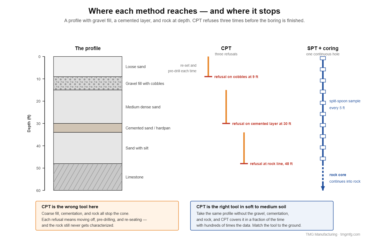
    • Continuous profiling. SPT is a discrete test. Thin layers need CPT or continuous sampling.
    • Tripod and hand-hammer setups. Genuinely useful for limited-access work, and we sell them — but D1586 §1.7 frames the test around rotary drilling equipment and the standard does not address hand driving. Report tripod results as penetration resistance data with that qualification, not as D1586 N-values.

    Standards Status: Check Your Boilerplate

    As of August 2026, ASTM has withdrawn much of the field sampling suite that boring-log legends habitually cite — most out of subcommittee D18.02, with RQD going the same way out of D18.12:

    StandardSubjectStatus (Aug 2026)
    D1586/D1586M-18e1SPT and split-barrel samplingActive (revision work item WK99626 open)
    D6151-25Hollow-stem augersActive (reinstated; “M” dropped)
    D5434-25Field logging of subsurface explorationsActive (reinstated)
    D2488-26Visual-manual descriptionActive
    D2487-17(2025)USCS classificationActive
    D5783-18(2025)Direct rotary, water-based fluidActive
    D6286/D6286M-20Selection of drilling and direct push methodsActive
    D1587/D1587M-15Thin-walled tube samplingWithdrawn 2024
    D2113-14Rock core drillingWithdrawn 2023
    D4220/D4220M-14Preserving and transporting soil samplesWithdrawn 2023
    D4633-16Energy measurement for dynamic penetrometersWithdrawn 2025
    D6066-11Normalized penetration resistance of sandsWithdrawn 2020
    D6032/D6032M-17Rock quality designation (RQD)Withdrawn 2026

    A withdrawn standard is not a wrong method — it is a document ASTM no longer maintains. But writing “sampling per ASTM D1587, core per D2113, energy per D4633” into a 2026 specification means contractually referencing documents that are no longer current standards. Update the boilerplate, or name the method and edition explicitly.

    Common Mistakes That Ruin N-Values

    • Marking the rod from a nominal depth instead of the actual seated position.
    • Reporting only the sum instead of all three increment counts.
    • Logging “REF” instead of the partial penetration (write 50/3″).
    • Sampling into slough, or running a dented drive shoe for a whole boring.
    • Mixing upset-wall, constant-ID, and lined spoons in one project without noting it.
    • Comparing N-values across rigs with different hammers and no energy data.
    Four SPT field errors that produce a wrong N-value
    Figure 5. Slough, lost head, gravel on the shoe, and cathead wraps — and which way each biases N.

    What This Actually Costs You Downstream

    Pile capacity, settlement, liquefaction triage, shallow footings or deep foundations — all of it correlated from N. We size helical piles and underpinning products off boring logs every week, and the logs that cause problems are never the ones with bad-looking numbers. They are the ones with clean-looking numbers produced by a procedure nobody documented. Record the increments, the hammer, and how you reached depth, and the engineer can work with whatever the soil gave you.


    Need SPT equipment or a rig that runs the test properly? TMG Manufacturing builds SPT and coring rigs, automatic and manual safety hammers, split-spoon samplers, and sampler baskets, and tripods and capstans — and we repair hydraulic drill rigs regardless of who built them. Call (813) 464-2299 or toll-free 1-888-508-RIGS, or email info@tmgmfg.com.

    Ramzy Moumneh, TMG Manufacturing

    Frequently Asked Questions

    What is a good N-value in SPT testing?

    It depends on soil type and what you are building. Terzaghi and Peck’s ranges for sands: below 4 very loose, 4 to 10 loose, 10 to 30 medium dense, 30 to 50 dense, above 50 very dense. In clays, below 4 is soft and above 30 is hard. Correct field N to N60 before applying any published correlation.

    Why is the first 6 inches of an SPT not counted?

    The bottom of a borehole is disturbed by drilling, and the first 6 inches pushes the sampler through that disturbed zone — the seating drive. Counting it would mix drilling disturbance into a soil measurement, so D1586 discards it and defines N over the 0.5 to 1.5 ft portion of the drive.

    How deep should SPT borings go?

    Deep enough that the added stress from the foundation is negligible. The ASCE (1972) rule takes the shallower of two depths: where added vertical stress falls below about 10 percent of the applied pressure, and where it falls below 5 percent of the effective overburden stress. For deep foundations, extend well below the anticipated tip. The registered design professional sets the depth, not the driller.

    What is the difference between N and N60?

    N is the raw field blow count. N60 adjusts it to a drill rod energy transfer ratio of 60 percent of the theoretical 350 ft-lb: N60 = N × (ETR / 60). Because measured ETR runs from roughly 35 percent on a tired manual hammer to over 90 percent on a modern automatic, the two can differ by more than 30 percent on the same soil.

    Can you perform SPT without a drill rig?

    You can drive a split spoon with a tripod, a capstan, and a manual safety hammer, and it is useful for limited-access, interior, and remote work. What you cannot do is call the result an ASTM D1586 N-value — the standard frames the test around rotary drilling equipment and does not address hand driving. Report the data with that qualification.

  • CPT vs. SPT: How to Choose the Right Soil Test

    CPT vs. SPT: How to Choose the Right Soil Test

    CPT (cone penetration testing) pushes an instrumented cone continuously into the ground and returns a near-continuous profile of soil behavior, but recovers no sample. SPT (standard penetration test) drives a split-spoon sampler at intervals and returns both a blow count and a physical sample. CPT gives you more data; SPT gives you soil you can hold.

    That’s the short answer. The longer answer is that CPT vs SPT isn’t really a competition — the two tests answer different questions, and the projects that go badly are usually the ones where somebody picked a method to fit a budget instead of to fit the ground.

    We build both. TMG manufactures SPT and coring rigs and CPT and DMT test rigs out of Tampa, and we sell the cone equipment that goes on them. We have no reason to talk you into one over the other, which is more than most sources on this question can say.

    What each test actually measures

    The SPT is a dynamic test. A 140-pound hammer falls 30 inches onto a drill rod, driving a 2-inch outside-diameter split-barrel sampler into the soil at the bottom of a borehole. You count the blows for each of three 6-inch increments; the sum of the second and third is the N-value. The procedure is governed by ASTM D1586/D1586M-18e1. Then you open the sampler and you have real soil — enough to classify it, run Atterberg limits, check moisture content, or send it out for corrosivity testing.

    The CPT is a quasi-static test. A cone with a 60-degree apex — 10 cm² projected tip area is the reference size, 15 cm² is common in production work — is pushed into the ground at 20 ± 5 millimeters per second behind a matched friction sleeve (150 cm² on a 10 cm² cone). Load cells record tip resistance (qc), sleeve friction (fs), and, on a piezocone, pore water pressure (u2). ASTM D5778-20 requires readings at depth intervals no greater than 50 mm; most systems log every 2 centimeters. Nothing comes back up.

    CPT vs SPT diagram showing an SPT hammer driving a split-spoon sampler in a borehole beside a CPT cone pushed continuously into undisturbed ground
    The core difference in CPT vs SPT: the SPT drives a sampler in an open borehole and recovers soil; the CPT pushes an instrumented cone through ground it never disturbs.

    The difference in data density is what most people underestimate. A boring with SPT sampling at 5-foot intervals gives you roughly 20 N-values in 100 feet. A CPT sounding over the same 100 feet gives you well over a thousand readings across three independent measurements. Thin layers — a 6-inch clay seam, a loose lens in otherwise dense sand — are effectively invisible to a 5-foot sampling interval and unmistakable on a CPT trace.

    CPT vs SPT data density comparison showing a 7-inch soft clay seam captured by the continuous CPT trace but missed between 5-foot SPT sampling intervals
    A 7-inch soft seam at 21.5 ft. The CPT trace drops to under 1 MPa and recovers within eight inches. The SPT samples above and below it never touch the layer.

    Side-by-side comparison

    CPTSPT
    Governing standardASTM D5778-20ASTM D1586/D1586M-18e1
    Data intervalContinuous (≤50 mm required; ~2 cm typical)Discrete, typically 5 ft
    Soil sample recoveredNoYes — disturbed split-spoon sample
    Production rate~400–600 ft/day~160 ft/day (hollow-stem auger, 5-ft sampling)
    Operator dependenceLow — mechanized push, calibrated load cellsHigh — hammer type, rod length, borehole condition all affect N
    RepeatabilityExcellentModerate; requires correction factors
    Works in gravel, cobbles, fill, rockNo — refusalYes, within limits; coring for rock
    Detects thin layersYesUsually not
    Direct pore pressure measurementYes (piezocone)No
    Reaction required15–25 tons of rig or ballast weightRig weight, often supplemented with screw anchors
    Lab testing on recovered soilNot possible from the soundingYes

    Production rate figures follow Peter Robertson’s published comparison. His cost example — written in 2006 for the California market — put 400 feet of CPT at roughly $3,500 including plots and interpretation, against about $8,000 for three days of auger drilling plus lab cost on some 80 samples. Both figures are roughly 1.6 times higher in today’s dollars, and your local market will differ, but the ratio has held up: CPT is usually cheaper per foot of information and more expensive per day of rig time.

    The N-value problem nobody mentions until the design is done

    An N-value is not a soil property. It’s a measurement of how hard it was to drive a sampler with a particular hammer, through a particular rod string, in a particular borehole, on a particular day.

    The energy actually delivered to the rods varies enormously with hammer type. Measured fleet averages put automatic hammers around 75 to 90 percent of theoretical energy, clustering near 80 — the Vermont and North Carolina DOT studies both land there. A safety hammer runs roughly 55 to 70 percent. An old donut hammer can fall below 50 percent.

    Here’s the part clients get backwards: a low-energy hammer reports a higher N-value in identical soil, because it takes more blows to drive the sampler the same distance. Automatic versus safety hammers typically differ by about 40 percent. Automatic versus an old donut hammer can approach a factor of two — for the same ground.

    Chart comparing automatic, safety, and donut SPT hammer energy transfer and the different N-values each reports in identical soil
    The weakest hammer produces the highest N-value. This is why hammer calibration matters before anyone trusts a blow count.

    That’s why the profession applies correction factors for hammer energy, rod length, borehole diameter, and sampler configuration to arrive at N60, then normalizes for overburden to get (N1)60. It works, but it depends on knowing your rig’s actual energy ratio, which means the hammer has to have been calibrated. A lot of them haven’t been.

    TMG STR-174 SPT and wireline coring drill rig
    TMG’s STR-174 — SPT sampling and wireline core drilling on one rig.

    CPT sidesteps this entirely. The cone is pushed at a controlled rate by a hydraulic ram, and the load cells are calibrated instruments. Two crews with two rigs on the same site should produce nearly the same log. That repeatability is CPT’s strongest argument, and it’s an argument about the equipment — which is why we take hammer calibration seriously on the rigs we build.

    Where CPT simply cannot go

    This is the part CPT vendors tend to leave out.

    Gravel, cobbles, and construction debris fill. A cone 3.6 to 4.4 centimeters across meeting a cobble either deflects or refuses. You get a spike in tip resistance and a sounding that stops well short of target depth.

    Cemented sands and hardpan. Common in parts of Florida, and a frequent cause of premature refusal.

    Rock. CPT cannot characterize rock at all. If the structure bears on rock, you need core. Rock coring was long governed by ASTM D2113, which ASTM withdrew in 2023 without a replacement; it is still named in some codes and remains the de facto reference in practice. Depth rules vary by jurisdiction — the model IBC (§1803.5.6) requires borings at least 10 feet below foundation level where rock structure varies, while New York City is more prescriptive, calling for a double-tube core barrel of at least 2⅞ inches outside diameter cored no less than 10 feet below the lowest level of bearing.

    Sites without reaction. A CPT rig has to push against its own weight. Most production units run 15 to 25 tons. On a site with poor access, soft ground, or overhead restrictions, that mass may simply not be deliverable — and a lighter rig will lift off the ground before it reaches depth.

    Anywhere you need the soil itself. Classification, plasticity, organic content, contamination screening, corrosivity for buried steel — all of it requires a sample. This matters directly if you’re designing helical piles or any other steel deep foundation, where soil resistivity, pH, and chloride content drive the corrosion allowance and the galvanizing specification.

    Soil profile diagram showing CPT refusing on cobbles, a cemented layer, and rock while a single SPT boring with rock coring reaches full depth
    Three refusals in one profile. Each one means moving off, pre-drilling, and re-seating — and the rock still never gets characterized.

    What the building code actually says

    Worth knowing, and worth getting right: the model International Building Code does not address CPT at all. The words “cone” and “sounding” do not appear in Chapter 18. The IBC leaves the scope of investigation to the geotechnical engineer of record and the building official.

    Some jurisdictions are far more specific. New York City Building Code §1803.5.2, “Alternative Investigative Methods,” states that CPTs may replace borings on a one-to-one basis, but in no case shall there be fewer than half the required standard borings, and no less than two standard borings — and it further requires that boring depth requirements be met with borings, not soundings.

    That’s a useful model even where it isn’t law. The one code that bothered to write a rule did not treat CPT as a full substitute; it treated it as a method that can carry half the load. If your plan calls for eight borings, you can run four borings and four soundings — not eight soundings.

    Florida follows the model IBC here, with no CPT provision. So in most of the country this is an engineering-judgment call, not a compliance checkbox. Check your AHJ before assuming either way.

    CPT vs SPT: how to actually choose

    Lean CPT when: the site is soft to medium soil with no gravel; you need to find thin compressible layers; settlement prediction governs; you have a lot of ground to cover on a schedule; or you need pore pressure data. CPT-based liquefaction triggering procedures are well established, and the continuous profile resolves thin liquefiable layers that 5-foot sampling misses — though SPT-based procedures are equally current, and the two are often run together as a cross-check.

    TMG CPT-223 CPT and DMT test rig ready for a geotechnical soil investigation
    TMG’s CPT-223 — a dedicated CPT and DMT push rig for soft to medium ground.

    Lean SPT when: the profile includes gravel, cobbles, fill, or rock; you need samples for lab classification or corrosivity; the design is driven by an N-value correlation your reviewer expects to see; access is tight and you can’t get reaction weight on site; or local practice and the AHJ expect borings.

    Use both when the project is large enough to matter — which is most of them. The efficient pattern is to run CPT soundings to map the site quickly and continuously, then place a smaller number of borings at the critical locations the CPT identifies, sampling where the profile actually changes rather than every 5 feet by default. You get continuous coverage and the samples the lab needs, usually for less than either approach alone done to the same confidence.

    TMG CSR-174 combination rig that performs both CPT soundings and SPT borings
    When the answer is both, one machine can do both. TMG’s CSR-174 runs CPT soundings, SPT sampling, wireline coring, and rotary drilling.

    Why this shows up in your foundation design

    The CPT vs SPT decision eventually lands on a pile schedule. If you’re sizing helical piles, the CPT trace tells you where the competent bearing stratum starts and how consistent it is across the site — which determines helix depth and whether one configuration works everywhere or you need two. The SPT samples tell you what that stratum is made of, and whether the groundwater chemistry is going to eat galvanizing in twenty years.

    Neither test alone gets you there. That’s the whole point. Once you have the profile, our Helical Pier Load Calculator is a quick way to sanity-check a configuration before it goes on a drawing.


    Questions about which rig configuration fits your work? TMG builds SPT and coring rigs, CPT and DMT test rigs, and the cone equipment that goes with them — and we repair hydraulic drill rigs regardless of who made them. Call (813) 464-2299, toll-free 1-888-508-RIGS, or email info@tmgmfg.com.

    Ramzy Moumneh is the founder of TMG Manufacturing in Tampa, Florida, which builds geotechnical drill rigs and deep foundation products.

    Frequently asked questions

    Is CPT more accurate than SPT?

    CPT is more repeatable and far more continuous, so it produces a more reliable picture of how soil properties change with depth. SPT is more versatile — it works in ground where CPT refuses, and it recovers a sample. “Accurate” depends on which question you’re asking.

    Can CPT replace SPT entirely?

    Rarely in practice, and in some jurisdictions not legally. The model IBC is silent on CPT and leaves the call to the engineer of record and the building official. New York City is explicit: CPTs may replace borings one-for-one, but at least half the required standard borings — and never fewer than two — must remain, and boring depth requirements must be met with borings.

    How deep can a CPT go?

    Depth is limited by reaction weight and soil resistance rather than by the equipment itself. A 20-ton rig commonly reaches 150 feet or more in soft to medium soils, and refuses much shallower in dense sand or gravel.

    Why do two crews get different N-values in the same soil?

    Mostly hammer energy. A low-energy hammer has to hit more times to drive the sampler the same distance, so it reports a higher N in identical soil. Automatic versus safety hammers typically differ by about 40 percent; automatic versus an old donut hammer can approach a factor of two. That’s what the N60 correction exists to fix.

    Do I need a sample if I have CPT data?

    Yes, if you need soil classification, Atterberg limits, organic or contaminant screening, or corrosivity testing for buried steel. CPT infers soil behavior type; it does not recover soil.