Category: Helical Piles

Take the bearing stratum depth and N-value off the log, correct N for hammer energy and overburden, convert to a friction angle, compute effective overburden stress at each helix using buoyant unit weights, and sum Ah·q’·Nq across the plates. Divide the required ultimate by Kt and you have the installation torque to write on the drawing.

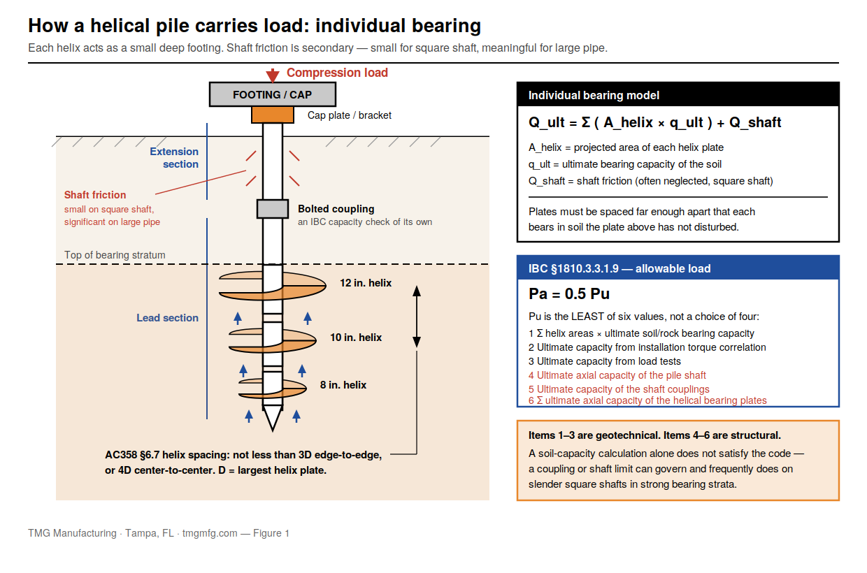
That is the workflow, and it is not just convention — it is IBC §1810.3.3.1.9, which sets the allowable axial load of a helical pile at Pa = 0.5 Pu (Equation 18-4) and defines Pu as the least of several quantities, the first being the sum of the areas of the helical bearing plates times the ultimate bearing capacity of the soil. Florida adopts the model IBC deep-foundation provisions through the Florida Building Code. The factor of safety of 2 you have seen your whole career is that 0.5.

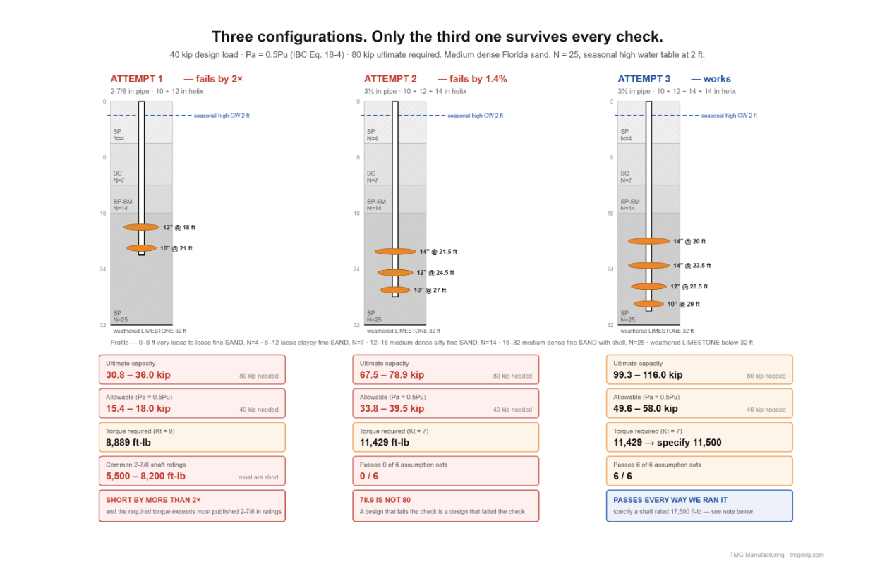
This post runs the method end to end on a realistic west-central Florida profile. The first configuration we try fails by a factor of two. The second one gets within a percent and a half of passing — and still fails, on every assumption we test it against. Only the third works. That sequence is the useful part. A clean worked example teaches you the arithmetic; a failed one teaches you where the arithmetic bites.

We build both the rigs that produce these logs and the piles designed from them, which is the only reason we can write this particular post.

What a pile designer actually uses

Column	What it’s for
Depth and layer boundaries	Sets helix elevations, defines top and bottom of the bearing stratum
N-value — all three 6-inch increments	Source of φ and Su. Never use only the summed N; the increments reveal shell and gravel spikes and weight-of-rod zones
USCS symbol and description	Decides whether you’re on the drained branch (φ, Nq) or the undrained one (Su, Nc = 9)
Groundwater — at drilling, at 24 hours, seasonal high	Effective overburden. In sand this drives capacity directly
Sample recovery	Zero recovery is data — raveling, running sand, or a void
Drilling notes	Fluid loss and “fell by weight of rod” are karst indicators
Termination depth	A hard constraint. You cannot design a helix below the depth you explored

Largely ignored for capacity: moisture content, Atterberg limits except to pick a correlation and flag organics, and the minus-200 fraction beyond classification.

What makes a stratum worth bearing in

Worth separating what the code says from what is judgment, because most published lists blur them:

Criterion	Value	Status
Allowable load = half the ultimate	Pa = 0.5 Pu	Code — IBC §1810.3.3.1.9, Eq. 18-4
Firm soil for bearing and lateral support	N ≥ 5	Code-adjacent — AC358 §3.11.2.1 defines firm N≥5, soft 0<N<5, fluid N=0
Practical minimum for a helix bearing layer	N ≥ 10–15 sand, 8–10 clay	Judgment — in no code
Inter-helix spacing	3 × diameter of the lower plate	Industry practice — stated in the ESRs, not in the IBC. AC358 Table 3 sets 2.4D–3.6D as the conformance window for using the default Kt
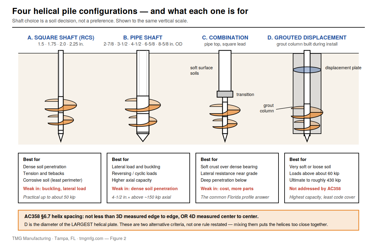
Pile-to-pile spacing before group effects	3D clear / 4D center-to-center	Code-adjacent — AC358 §6.7 (this is the pile spacing rule, often misquoted as the helix rule)
Uppermost helix depth in tension	≥ 12 × largest helix diameter	Code-adjacent — AC358 §4.4.1.1, §6.9, tension only
Bearing layer thickness below the lead helix	≥ 3 × helix diameter commonly cited	Judgment — no code number exists
Depth for “deep” bearing behavior	> 5 × largest helix diameter	Practice
Same bearing layer present in every boring	—	Judgment, and the most violated rule

Three borings, one site, three different answers

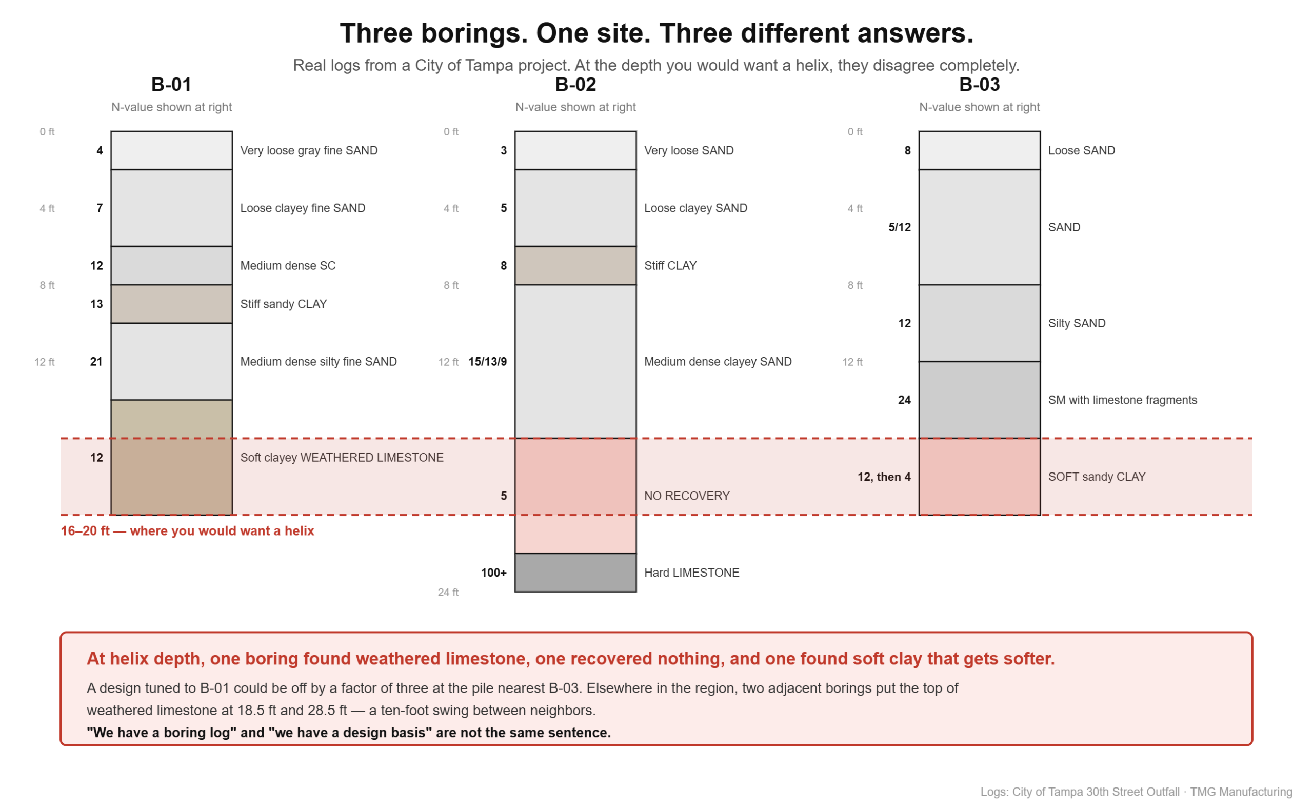
Before any arithmetic, the thing that should worry you most. These are real borings from a City of Tampa project, all on one site:

Depth 16–20 ft	B-01	B-02	B-03
Material	Soft clayey weathered limestone	No recovery	Soft sandy clay
N-value	12	5	12, then 4

At the depth where you would want your helix, one boring found weathered limestone, one recovered nothing at all, and one found soft clay that gets softer. A design tuned to B-01 could be off by a factor of three at the pile nearest B-03.

Another regional example: two adjacent borings where the top of weathered limestone varied from 18.5 ft to 28.5 ft — a ten-foot swing between neighbors.

This is the Florida condition, and it is why “we have a boring log” and “we have a design basis” are not the same sentence.

From N-value to soil parameters

Correct N first

Published correlations are written for N60 — N corrected to 60% hammer energy. Field N is not N60.

N60 = N × (hammer efficiency / 60), with adjustments for borehole diameter, sampler, and rod length. Automatic hammers commonly run 75–85% efficiency; safety hammers 55–60%.

The correction does not always go up. An automatic hammer at 80% turns a field N of 25 into N60 ≈ 33 — a 33% increase. A safety hammer at 55% turns that same field N of 25 into N60 ≈ 23 — a decrease. Which direction you move depends entirely on the hammer, and the hammer is in the report’s methodology section, if it is stated at all. Assuming every correction is upward is how you end up unconservative on a safety-hammer log. (We wrote a whole post on why that number moves so much.)

For granular soils you then normalize for overburden: CN = √(Pa/σ’v0), giving (N1)60. Because Florida water tables are shallow, effective stress is low and CN often lands between 1.3 and 1.7 at helix depth — a large upward correction.

Then convert — and look at the spread

At our example point — field N = 25, safety hammer taken at 60% so N60 = 25, effective overburden 1,058 psf, giving CN = 1.41 and (N1)60 = 35:

Correlation	Argument	φ
Peck-Hanson-Thornburn (Wolff 1989 fit)	(N1)60 = 35	37.0°
Peck-Hanson-Thornburn (Wolff 1989 fit)	N60 = 25	34.3°
Industry helical correlation, φ = 0.28N + 27.4	N = 25	34.4°
Hatanaka & Uchida (1996), φ = √(20·(N1)60) + 20	(N1)60 = 35	46.6°
Kulhawy & Mayne (1990)	N60 = 25, σ’v/Pa = 0.50	46.1°

A 12-degree spread from one N-value. Because Nq is exponential in φ, going from 34° to 46.6° is a factor of more than five on computed helix capacity. Note also that Hatanaka & Uchida is defined on (N1)60, not N60 — feeding it raw N60 is a common error that lands you about 4° low and quietly looks reasonable.

Hatanaka & Uchida and Kulhawy & Mayne are known to run high for fine, rounded, uniform quartz sands — which is exactly what Florida has. Most Florida practitioners cap φ at 32–35° for medium dense fine sand regardless of what the correlation returns. That cap is judgment, not derivation, and anyone presenting it as a calculation is overselling it.

We will design at φ = 34°, the value the two conservative correlations agree on. Note what that means: we normalize N for overburden to see the spread, then design off the un-normalized branch. That is deliberate and conservative — using (N1)60 = 35 would give φ = 37° and about 46% more capacity — but it should be stated, not buried, because a reviewer will ask which one you used.

For clays, Su ≈ 125·N psf is the traditional relation. Treat it with real suspicion. Reid and Taylor’s re-analysis of the underlying dataset (Ground Engineering, July 2010) found the multiplier ranging from 0.18 to 19.30 kPa per blow with R² below 0.2 — no significant association at all. Their mean of about 4 kPa/blow is roughly 84 psf/blow, which puts the traditional 125 psf/blow (≈ 6 kPa/blow) about 50% above the re-analyzed mean — the unconservative side. Use SPT-to-Su in soft clay for screening. For design, get a load test or a CPT cross-check.

The profile

A composite that reflects what Tampa-area logs actually show:

Depth (ft)	Description	USCS	N	γ moist	γ sat
0–6	Very loose to loose fine SAND	SP	4	105	110
6–12	Loose clayey fine SAND	SC	7	110	115
12–16	Medium dense silty fine SAND	SP-SM	14	112	118
16–32	Medium dense fine SAND with shell	SP	25	115	122
32+	Weathered LIMESTONE	—	15–50+	—	—

Water table measured at 4 ft; seasonal high estimated at 2 ft. Boring terminated at 35 ft.

We design to the seasonal high, not the measured reading. Every effective stress below is computed with the water table at 2 ft. This costs about 7% of capacity relative to the 4-ft reading, and it is not optional — a March boring in Tampa is not the condition your pile will see in September.

Effective overburden, buoyant below the water table:

q'(18 ft) = 2(105) + 4(110−62.4) + 6(115−62.4) + 4(118−62.4) + 2(122−62.4)
          = 1,058 psf
q'(20)=1,177   q'(21)=1,236   q'(21.5)=1,266   q'(23.5)=1,385
q'(24.5)=1,445  q'(26.5)=1,564  q'(27)=1,594   q'(29)=1,713 psf

Which Nq

Two equations are in common use in the helical industry, and neither is more official than the other:

• Perko (2009), after Meyerhof: Nq = 0.5(12φ)^(φ/54) → 22.0 at 34°
• A variant widely used in the industry’s technical literature, which adds a unity term: Nq = 1 + 0.56(12φ)^(φ/54) → 25.7 at 34°

A 17% swing before any soil variability is considered. We carry both through every calculation below. A design that only works on the friendlier of two equally citable equations is not a design.

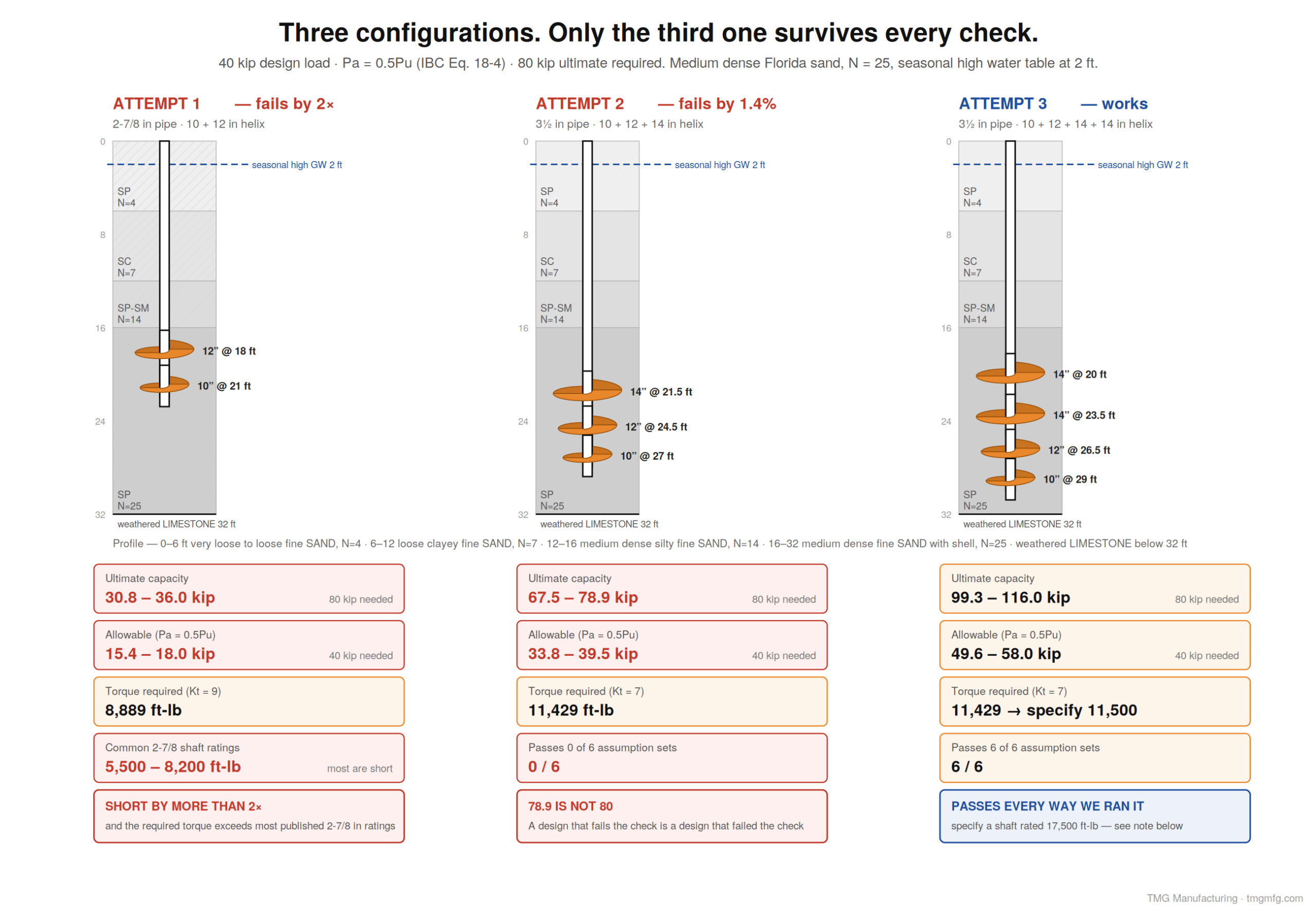
Attempt one — short by a factor of two

Design load 40 kip compression. Pa = 0.5Pu, so we need 80 kip ultimate.

Try a 2⅞-inch pipe shaft with a 10-inch lead at 21 ft and a 12-inch upper at 18 ft — 3.0 ft apart, which clears 3D on the lower (10-inch) plate, 2.5 ft. Net projected areas, plate minus shaft: 12 in = 0.740 ft², 10 in = 0.500 ft².

With Nq = 25.7:

12 in @ 18.0 ft : 0.740 × 1,058 × 25.7 = 20,122 lb
10 in @ 21.0 ft : 0.500 × 1,236 × 25.7 = 15,898 lb
                                  Qult = 36,020 lb = 36.0 kip
                                Qallow = 18.0 kip

With Nq = 22.0: Qult = 30.8 kip, Qallow = 15.4 kip.

We needed 80 kip ultimate. We have 31 to 36. Short by more than a factor of two.

Run it backwards to see how far off:

Required average unit bearing = 80,000 / 1.241 ft² = 64,482 psf
Area-weighted average q' across the two helices = 1,130 psf
Required Nq = 64,482 / 1,130 = 57.1   →  φ ≈ 40–41°

N = 25 does not produce φ = 41° in Florida fine sand under any correlation a reviewer would accept.

It fails a second time, independently

T required = 80,000 / 9 = 8,889 ft-lb

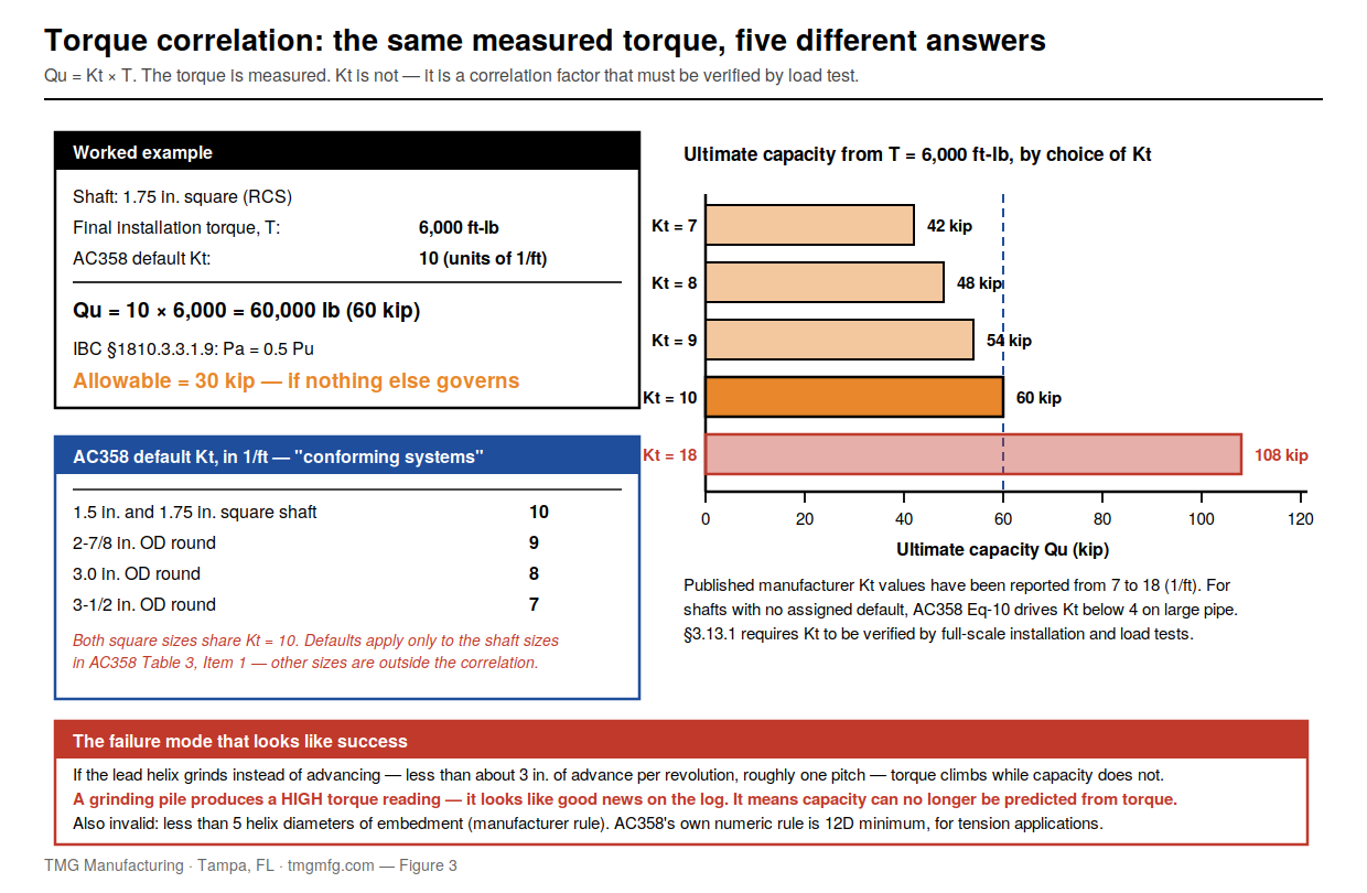
Kt = 9 ft⁻¹ for 2.875-inch round shafts, per AC358 §3.13.1.1.

Torque ratings for 2⅞-inch round shafts published in ICC-ES evaluation reports and manufacturer data run from about 5,500 ft-lb through 6,400, 7,900, and 8,000 to 8,200 ft-lb, varying with wall thickness and coupling type, with one heavier-wall product rated 11,000. Most of the common ones sit below 8,889.

Take a shaft rated 8,000 ft-lb: 8,000 × 9 = 72 kip ultimate, 36 kip allowable — below the 40 kip design load before soil is considered at all.

Two independent checks, both failing. That is the useful signal. When the bearing calculation and the torque calculation disagree with your load, they are usually agreeing with each other.

Note what they actually say here: the computed soil capacity of 36.0 kip implies 36,000 / 9 = 4,000 ft-lb of installation torque, which is about what a 10/12 on 2⅞-inch pipe really reads in medium dense Florida sand. The methods agree. The load is the problem.

(One honesty note on that cross-check: the bearing sum counts only the helices, while the torque correlation predicts total pile capacity including shaft friction over 21 feet of soil. They are not the same quantity. The bearing sum is the conservative one, and the agreement here is close enough to be informative, not close enough to be a proof.)

Attempt two — one and a half percent short, which is still short

Go up a shaft size and add a plate. 3½-inch pipe, triple helix 10/12/14: 10-inch lead at 27 ft, 12-inch at 24.5 ft, 14-inch at 21.5 ft. Spacings are 2.5 ft and 3.0 ft, which is 3D off each lower plate, and this is a real manufactured lead-section geometry.

                                        Nq = 25.7        Nq = 22.0
10 in @ 27.0 ft : 0.479 × 1,594 ×  →     19,606 lb        16,784 lb
12 in @ 24.5 ft : 0.719 × 1,445 ×  →     26,686 lb        22,844 lb
14 in @ 21.5 ft : 1.002 × 1,266 ×  →     32,613 lb        27,918 lb
                             Qult  =     78.9 kip         67.5 kip

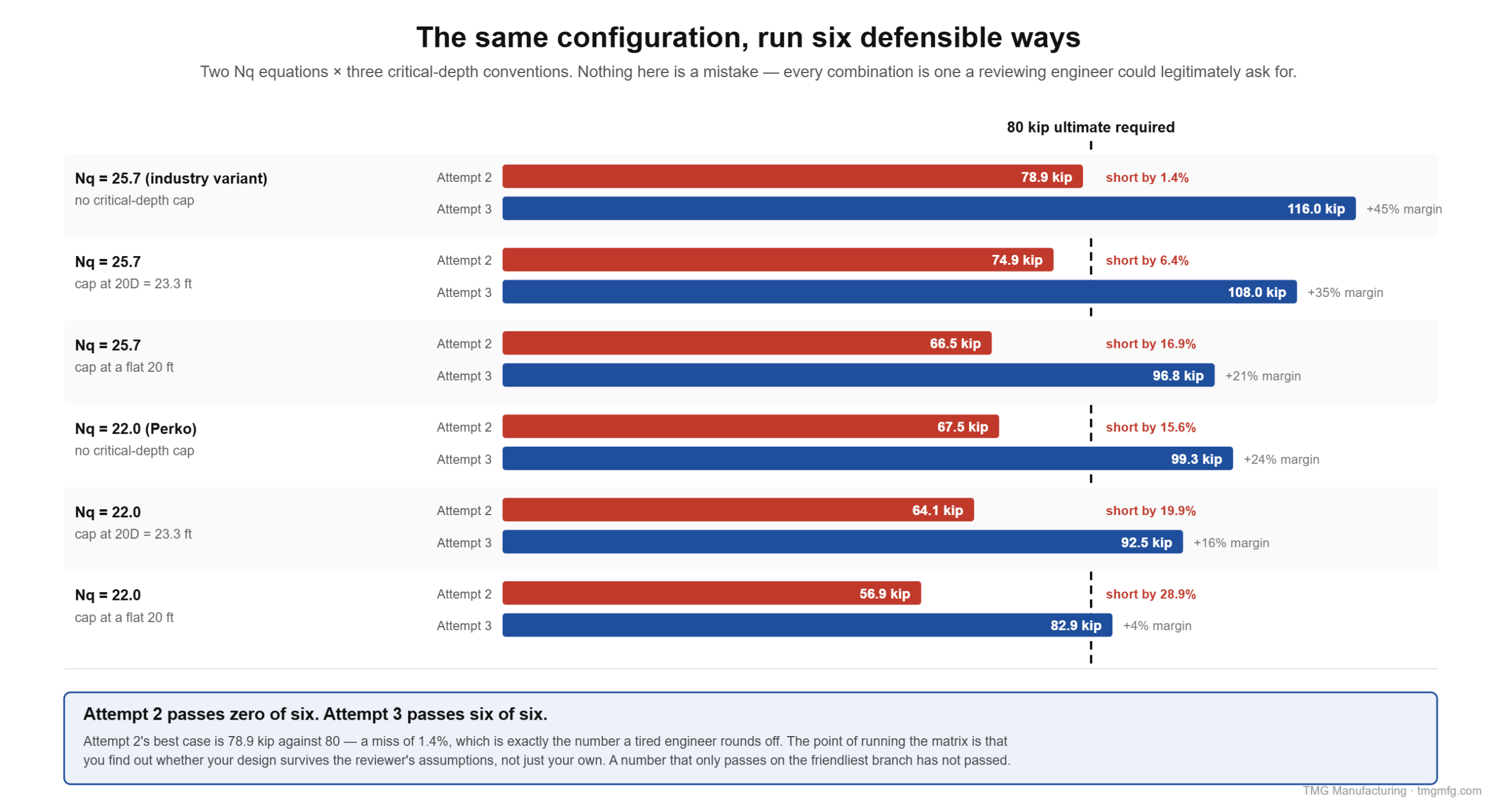
78.9 against 80 needed. On the more favorable of the two Nq equations, at no critical-depth cap, this configuration misses by 1.4%. On the other equation it misses by 16%.

78.9 rounds to 79, 79 is “basically 80,” and the temptation to call it close enough is real — particularly when the number came out of a spreadsheet. A design that fails the check is a design that failed the check. And this one fails on every branch we can test: two Nq equations times three critical-depth conventions is six defensible ways to run the same configuration, and it misses all six, by 1.4% at best and 29% at worst. Go bigger.

Attempt three — a configuration that works

3½-inch pipe, four helices 10/12/14/14: 10-inch lead at 29 ft, 12-inch at 26.5 ft, 14-inch at 23.5 ft, 14-inch at 20 ft. Spacings of 2.5, 3.0, and 3.5 ft — 3D off each lower plate, all within AC358 Table 3’s 2.4D–3.6D window for using the default Kt.

                                        Nq = 25.7        Nq = 22.0
10 in @ 29.0 ft : 0.479 × 1,713 ×  →     21,072 lb        18,039 lb
12 in @ 26.5 ft : 0.719 × 1,564 ×  →     28,887 lb        24,728 lb
14 in @ 23.5 ft : 1.002 × 1,385 ×  →     35,683 lb        30,546 lb
14 in @ 20.0 ft : 1.002 × 1,177 ×  →     30,310 lb        25,947 lb
                             Qult  =     116.0 kip        99.3 kip
                           Qallow  =     58.0 kip         49.6 kip

Now the same six-way check, side by side with Attempt two:

Nq	Critical-depth cap	Attempt 2	Attempt 3
25.7	none	78.9 ✗	116.0 ✓
25.7	20D = 23.3 ft	74.9 ✗	108.0 ✓
25.7	flat 20 ft	66.5 ✗	96.8 ✓
22.0	none	67.5 ✗	99.3 ✓
22.0	20D = 23.3 ft	64.1 ✗	92.5 ✓
22.0	flat 20 ft	56.9 ✗	82.9 ✓

Zero for six, then six for six. Attempt three’s worst branch — conservative Nq, seasonal-high water table, and the most aggressive critical-depth cap anyone applies — still clears 80 kip. That is what a design you can defend in a plan review looks like: not a number that passes, a number that passes however the reviewer chooses to run it.

Other checks: bearing layer must extend at least 3D below the lead helix. On the lead (10-inch) plate that is 29 + 2.5 = 31.5 ft against a layer bottom at 32 ft — it clears, barely. On the largest (14-inch) plate it would be 32.5 ft, and it would not. The convention is not settled, so say which one you used, and treat 29 ft as the deepest lead elevation this profile supports.

Installation torque

T min = 80,000 / 7 = 11,429 ft-lb   →  specify 11,500 ft-lb

Kt = 7 ft⁻¹ for 3.5-inch round shafts, per AC358 §3.13.1.1. The bigger shaft has the lower correlation factor, which is why required torque goes up 29% while the shaft only went up 22% in diameter. This surprises people every time.

Now the shaft check, and it is not the one you expect. Published 3½-inch round shaft ratings cluster at 11,000, 13,000, 14,144, and 17,500 ft-lb across the current evaluation reports.

A 13,000 ft-lb shaft clears the 11,500 specification with 13% margin, so it looks fine. It is not. If the soil actually delivers the 99 kip our conservative branch predicts, the torque at 29 ft will read 99,300 / 7 ≈ 14,200 ft-lb — and more than that once shaft friction is counted. The installer hits the shaft’s torsional limit and refuses above design depth, and now you are on the phone arguing about whether a pile that stopped at 26 ft is acceptable.

Specify the 17,500 ft-lb shaft. The rule: your shaft rating has to cover the torque the soil will generate at your specified depth, not just the torque your capacity calculation requires.

The critical-depth caveat, stated honestly

Some offices cap effective overburden below a critical depth, on the reasoning that q’ stops increasing linearly in sand. The number matters enormously, and the commonly-repeated “20 feet” is not what the source says. The paper most often cited for it recommends 20D to 30D where D is the largest helix plate diameter, noting published values range from 10D to 40D.

For our 14-inch plate that is 23.3 to 35 ft — meaning at 30D no cap applies to this pile at all, while the flat 20-foot cap in our table is 17D, below the low end of the recommended range. We included it anyway, as the most punitive assumption available. State which convention you used. It is judgment, not derivation, and on a marginal design it decides the answer.

Writing the acceptance criterion

The output of all this is two numbers on a drawing:

Install to a minimum effective installation torque of 11,500 ft-lb, measured as the average over the final 3 feet of advance, and to a minimum lead-helix depth of 29 ft below existing grade.

Both conditions, not either. Torque alone is not enough — a pile can hit design torque in a two-foot dense crust at 8 ft and be nowhere near the bearing stratum. Depth alone is not enough either, because the stratum moves between borings.

Note the wording: lead-helix depth, not tip elevation. The lead helix on a manufactured lead section sits a few inches above the tip, so a “tip at 29 ft” instruction puts your bearing plate shallower than you designed it. And if you do write an elevation, name the datum.

Where this goes wrong

Each of these has a direction. Knowing which errors are safe and which are dangerous matters more than knowing the list.

Forgetting buoyancy — dangerous. Using total instead of effective unit weight below the water table in this profile takes q'(18) from 1,058 to 2,056 psf, nearly double, and Attempt one’s Qult from 36.0 to 70.3 kip. A 95% overestimate, in the direction that gets a foundation built on air.

Designing to the measured water table instead of the seasonal high — dangerous. In this profile it is about 7%. In a flatter one it is more.

Using uncorrected N-values — direction depends on the hammer. On an automatic hammer, raw N under-predicts and you leave capacity on the table — costly, not unsafe. On a safety hammer the correction runs the other way, and treating raw N as N60 is unconservative. Find the energy ratio before you decide which mistake you are making.

Feeding N60 into a correlation written for (N1)60 — conservative here, but wrong. Hatanaka & Uchida on N60 instead of (N1)60 gives about 42° instead of 47° in this profile. Safe direction, still an error, and it will be caught.

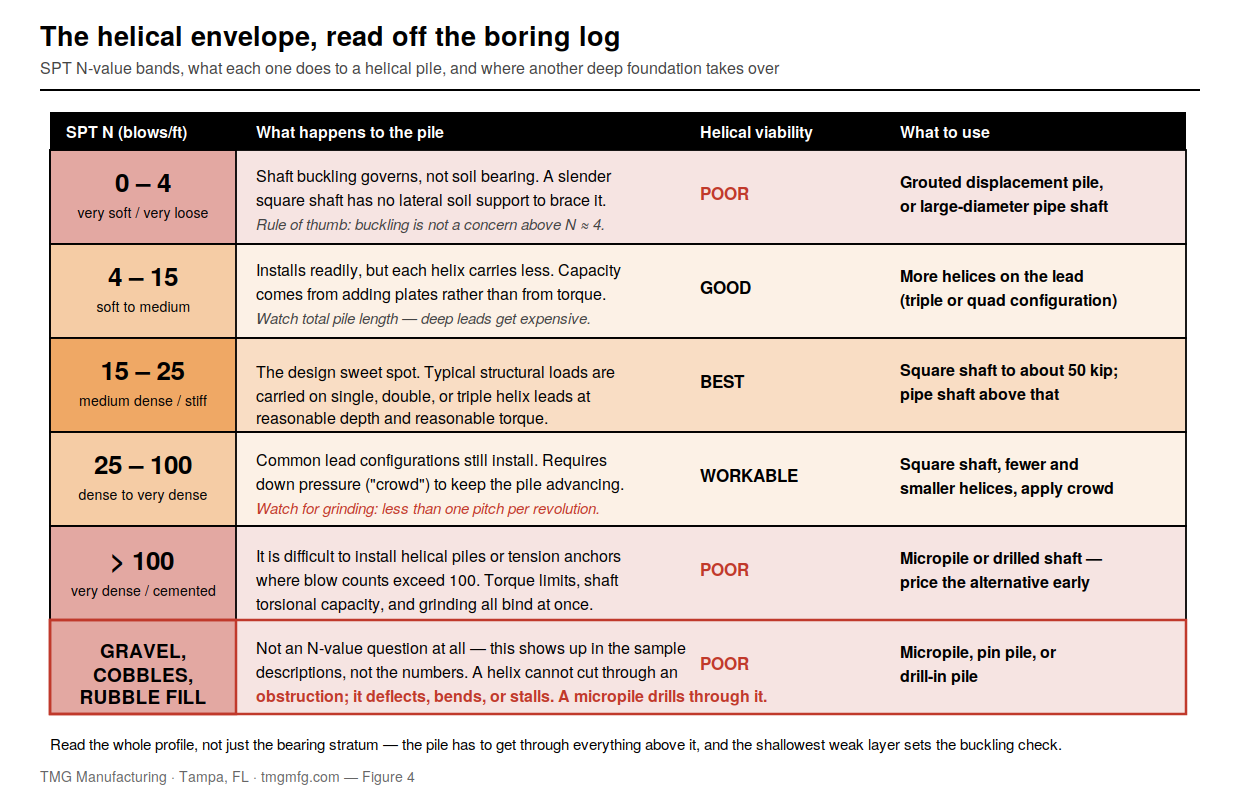
A bearing layer that’s too thin — dangerous. If a helix sits an inch above a change from dense to soft and you only compute at that elevation, the answer is derived entirely from the dense layer. Compute at the helix depth and one and two diameters below, and take the lowest. In Florida this bites specifically at the sand-over-weathered-limestone contact — where, as Tampa B-01 shows, “soft clayey weathered limestone, N=12” can be weaker than the sand above it.

Ignoring the shaft’s torque rating — dangerous in the field, not on paper. It does not make the pile weaker; it makes the pile stop short, which is worse because it happens at 4 p.m. with a crew standing around.

Skipping the buckling check — dangerous. With 6 to 12 ft of N = 4 to 7 over the bearing layer, this profile is exactly the case that needs one.

Designing below the boring — dangerous. Those Tampa borings stopped at 20 to 24 ft. Anything specified deeper is extrapolation, and our Attempt three at 29 ft would need a deeper boring than two of those three.

Trusting one boring — dangerous. See the three-boring table above.

What the log will not tell you

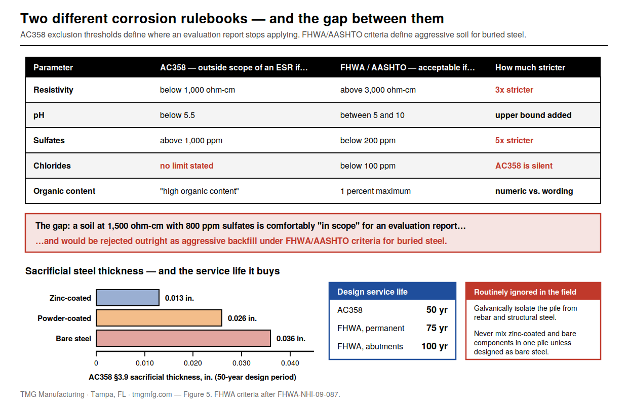
Corrosion parameters. A standard geotechnical boring log for a building foundation contains none of the electrochemical data a helical design needs: resistivity, pH, sulfates, chlorides, organic content. Those are separate tests that have to be requested — and on a coastal Florida site they are not optional.

Note also that thresholds disagree. AC358’s scope exclusions (§1.2.2) sit at resistivity below 1,000 ohm-cm, pH below 5.5, and sulfates above 1,000 ppm. The FHWA and AASHTO “non-aggressive” criteria are far stricter — 3,000 ohm-cm and 200 ppm. AC358’s numbers are a scope exclusion, not a design criterion, and citing them as though they were a pass mark is a common error.

Also absent: the hammer energy ratio, which moves φ by 5° or more. The seasonal high water table, often only estimated. The extent of any karst — SPT gives you circulation loss and weight-of-rod zones as indicators, not geometry. Whether the surficial soil is fill, and how old. And lateral variability, which is the whole point of the three-boring table.

---

Want a second set of eyes on a configuration? TMG manufactures helical piles, pile caps, brackets, and underpinning products in Tampa, and builds the SPT and CPT rigs that produce the logs behind them. Our Helical Pier Load Calculator is a quick way to check a configuration before it reaches a drawing. Call (813) 464-2299, toll-free 1-888-508-RIGS, or email info@tmgmfg.com.

Ramzy Moumneh, TMG Manufacturing — Tampa, Florida. TMG builds geotechnical drill rigs and deep foundation products.

---

FAQ

How do you size a helical pile from a boring log? Pick a bearing stratum with adequate N-value and thickness, compute effective overburden stress at each proposed helix depth using buoyant unit weights below the seasonal high water table, convert corrected N to a friction angle, and sum Ah(c·Nc + q’·Nq) across the plates. IBC Equation 18-4 then sets the allowable load at half that ultimate.

What N-value do you need for a helical pile bearing stratum? There is no code number. AC358 defines firm soil as N ≥ 5, which is a lateral-support threshold rather than a bearing criterion. Practical judgment puts a usable bearing layer at N ≥ 10 to 15 in sand and 8 to 10 in clay, with at least three helix diameters of that material below the lead plate.

Do you use raw N-values or corrected ones for helical pile design? Corrected. Published correlations are written for N60. The correction can go either way — an automatic hammer pushes N up by about a third, a safety hammer pulls it down — and because Nq is exponential in friction angle, either error moves computed capacity substantially.

How do you calculate the installation torque to specify? Divide the required ultimate capacity by the shaft’s Kt factor. AC358 §3.13.1.1 gives Kt = 9 ft⁻¹ for 2⅞-inch round shafts and 7 ft⁻¹ for 3½-inch, so 80 kip ultimate on a 3½-inch shaft requires about 11,400 ft-lb. Then check that number against the shaft’s published torsional rating — and against the torque the soil will actually generate at your design depth, which is usually higher.

Why does the water table matter so much for helical piles in Florida? Helix bearing capacity in sand is directly proportional to effective overburden stress. Below the water table, buoyancy roughly halves the effective unit weight. In a typical Tampa profile, using total stress instead of effective inflates computed capacity by about 95%.

---

Sources

• IBC §1810.3.3.1.9 and Equation 18-4 (allowable axial load of helical piles); adopted in Florida through the FBC deep-foundation provisions
• ICC-ES AC358, Acceptance Criteria for Helical Pile Systems and Devices — §1.2.2 (corrosion scope), §3.11.2.1 (soil definitions), §3.13.1.1 (Kt values), §4.4.1.1 and §6.9 (tension embedment), §6.7 (pile-to-pile spacing), Table 3 (helix spacing conformance window for default Kt)
• ICC-ES evaluation reports ESR-1854, ESR-3074, ESR-3418 and ESR-3982, and current manufacturer data sheets, for the published shaft torque ratings
• Perko, Helical Piles: A Practical Guide to Design and Installation (Wiley, 2009) — Nq = 0.5(12φ)^(φ/54), after Meyerhof (1976)
• Published industry technical literature on bearing capacity factors for helical pile design (Nq = 1 + 0.56(12φ)^(φ/54)) and on critical depth in sands (20D–30D of the largest plate)
• DFI Helical Pile Foundation Design Guide, 1st Edition (2019)
• Peck, Hanson & Thornburn (Wolff 1989 fit); Kulhawy & Mayne (1990); Hatanaka & Uchida (1996)
• Reid, A. and Taylor, J., “The misuse of SPTs in fine soils and the implications of Eurocode 7,” Ground Engineering, July 2010
• City of Tampa 30th Street Outfall and Spring Lake Stormsewer geotechnical reports; SWFWMD geotechnical report; FDOT District 7 SR-60 geotechnical memo and Central Florida Sinkhole Evaluation

Helical piles install fast, quiet, and vibration-free with small equipment, reach limited-access sites, and are the only deep foundation whose design capacity is routinely accepted from an installation-torque correlation written into code. They lose to micropiles and drilled shafts in gravel, cobbles, very dense soil, and aggressive soils.

That summary is deliberately two-sided, because a helical pile article that only lists advantages is useless to the person who signs the drawings. Helicals are an excellent tool inside their envelope and a poor one outside it, and the boundary is sharper than most marketing suggests.

TMG Manufacturing sits on both sides of this. We build the rigs that collect the subsurface data — SPT, coring, CPT and DMT push rigs — and we manufacture the helical piles, underpinning brackets, pin piles, drill-in piles, and micropile products designed from that data. When a boring log says a helical is the wrong answer, we are the ones selling the alternative. That is why the “cons” section is the longer one.

How a Helical Pile Carries Load

A helical pile is a steel shaft with one or more helix-shaped bearing plates welded to it, rotated into the ground by a hydraulic torque motor. Each helix advances roughly one pitch per revolution — about 3 inches — so the pile screws in rather than displacing soil laterally the way a driven pile does.

Load transfers two ways. The dominant mechanism is individual bearing: each plate acts as a small deep footing, and geotechnical capacity is the sum of the plates’ bearing capacities. The secondary mechanism is shaft friction — small for a square shaft, meaningful for large pipe. In tension the same helices work in uplift, which is why helicals dominate the tieback and guy anchor market.

Configurations and Shaft Sizes

• Square shaft (round-corner square, “RCS”). 1.5, 1.75, 2.0, and 2.25 in. Highest torque capacity per pound of steel, least soil disturbance, least perimeter exposed to corrosion, best penetration into dense soil. Weak in buckling and lateral load. Manufacturer guidance puts the practical sweet spot at working loads up to roughly 50 kips.
• Pipe shaft. 2⅞, 3½, 4½, 6⅝, and 8⅝ in. OD. Far better lateral and buckling resistance, more shaft friction, more capacity — manufacturers recommend the 4½ in. and larger line for axial loads above about 150 kips and lateral loads above about 5 kips.
• Combination. Pipe on top for lateral and buckling resistance, square lead for penetration. Common where soft surface soils overlie a dense bearing stratum.
• Grouted displacement pile. A displacement plate builds a grout column around the shaft as it advances. Manufacturer literature reaches into the 400-kip ultimate range, and it is the standard answer in very soft or loose soil where an ungrouted shaft would buckle.

Helix plates are spaced so each bears in relatively undisturbed soil. ICC-ES AC358 §6.7 states the rule as not less than 3D edge to edge, or 4D center to center, where D is the diameter of the largest helical plate. Those are two alternative criteria, not one rule restated — mixing them puts your helices too close together.

The Pros and Cons, Side by Side

Factor	Helical pile	Honest assessment
Installation speed	Piles per hour, not per day; immediate loading	Real advantage; often decides schedule-driven repairs
Installed cost	Low, in the right soil	Disappears fast in dense or gravelly soil where installation stalls
Vibration	Effectively none	Real advantage next to sensitive or historic structures
Noise	Hydraulic motor only; no impact	Real advantage in occupied buildings and residential work
Equipment size	Mini excavator, skid steer, or handheld	Often the only option in a basement or crawlspace
Capacity verification	Torque correlates to capacity	Unusual among deep foundations — but conditional and size-limited
Spoil generation	None	Advantage on contaminated or landfill sites
Tension capacity	Excellent	Best-in-class for uplift and tiebacks
Weather / groundwater	Installs saturated; no dewatering, no curing	Advantage in Florida-type conditions
Dense sand, gravel, cobbles	Poor	Stalls or grinds; often a hard stop
High-capacity loads	Limited on common shaft sizes	Torque verification drops out of AC358 scope on the largest shafts
Aggressive soils	Poor without design attention	50-year sacrificial basis; excluded outright below 1,000 ohm-cm
Buckling in very soft soil	Poor for slender shafts	Below about N = 4, buckling governs, not bearing
Public design guidance	Thin	No dedicated FHWA manual, no dedicated AASHTO LRFD section

Torque Correlation: The Advantage Nobody Else Has

Rotate a helical pile into the ground and the torque required to keep it turning is measured continuously by the installing equipment. That torque correlates to capacity:

Qu = Kt × T

where Qu is ultimate capacity, T is final installation torque, and Kt is a torque correlation factor in ft⁻¹. AC358 publishes defaults for “conforming systems”: 10 ft⁻¹ for both 1.5 in. and 1.75 in. square shaft, 9 ft⁻¹ for 2⅞ in. round, 8 ft⁻¹ for 3.0 in. round, 7 ft⁻¹ for 3½ in. round.

Very few deep foundations give you this. A drilled shaft gives you an integrity test, not a capacity, until you load-test it. Driven piles give dynamic formulas and PDA. A helical tells you at every location whether it reached the torque the design assumed — before the structure goes on it.

The Part Nobody Tells You: When Torque Correlation Lies

The defaults are not universal, and it is not “just use 10.” AC358 §3.13.1 requires Kt to be verified by full-scale field installation and load tests, and the published defaults still carry a verification testing schedule. They attach to specific shaft sizes only. For sizes without an assigned default, AC358 gives Kt = 22.285 (d_eff)^−0.9195, which drives Kt down sharply as the shaft grows — around 8.5 for a 2.0 in. square shaft and below 4 for large-diameter pipe. And the criteria are explicit that the correlation “applies only to shaft sizes described in Item 1 of Table 3. For shaft sizes that are outside of this prescribed range, this torque correlation is outside the scope of this criteria.” The high-capacity pipe configurations people reach for on big projects are precisely the ones where the torque-verification advantage loses its ICC-ES standing. No brochure says that.

It inverts when the helix grinds. If the lead helix hits a hard layer and advances substantially less than its pitch — under about 3 inches per revolution — torque climbs while capacity does not. Published guidance is blunt: grinding does not mean the pile will not carry its rated load; it means capacity can no longer be predicted from torque. This is the failure mode that matters most, because it produces a high torque reading, which looks like good news on the log.

It is invalid at shallow embedment. Manufacturer guidance requires the uppermost helix at least 5 helix diameters below grade in cohesive and fine granular soils. That 5D rule is a manufacturer rule, not code and not AC358 — AC358’s own numeric rule is 12D for tension applications, with anything shallower requiring a registered design professional to set the depth.

It is calibrated on clay. Kt = 10 performs well in cohesive soils and tends to be conservative in clean granular soils. In sand it may leave capacity on the table; in a soil the correlation was never calibrated for, it may do the opposite.

One citation warning. A frequently referenced ASCE Journal of Performance of Constructed Facilities paper on installation torque and axial capacity in cohesionless soils has been retracted by ASCE, and is still cited widely without any retraction notice. If a design basis on your desk rests on it, check the source.

What the Code Actually Requires

IBC §1810.3.3.1.9 governs helical pile allowable capacity, with the same section number in the 2021 and 2024 IBC. It is routinely described online as “four methods.” It is not. It sets Pa = 0.5 Pu (Equation 18-4), where Pu is the least of six values: (1) sum of helix plate areas × ultimate soil or rock bearing capacity; (2) ultimate capacity from well-documented correlations with installation torque; (3) ultimate capacity from load tests; (4) ultimate axial capacity of the pile shaft; (5) ultimate capacity of the shaft couplings; (6) sum of the ultimate axial capacity of the helical bearing plates. Items 1–3 are geotechnical, 4–6 structural, and 0.5 is a blanket factor of safety of 2 on whichever governs.

IBC §1810.3.1.5, the design-conditions provision for helical piles, is one sentence and imposes no helix geometry: helical piles “shall be designed and manufactured in accordance with accepted engineering practice to resist all stresses induced by installation into the ground and service loads.” Note the second half — installation stresses are a code requirement, not an afterthought. Helix spacing and geometry rules come from AC358 or a manufacturer, not from that section.

IBC §1810.4.11 requires a registered design professional to set embedment depth and torsional resistance criteria, and prohibits exceeding the pile’s maximum allowable installation torque. IBC §1705.9 requires continuous special inspection during installation — equipment, pile dimensions, tip elevations, final depth, final torque. It is a standalone section, not a row in a Table 1705 matrix, and was §1704.10 in the 2009 IBC.

AC358 (24), published April 2025, is the current acceptance criteria as of August 2026. It covers axial compression, axial tension, and lateral loads, and permits Seismic Design Categories D through F where §3.14 is satisfied — older evaluation reports limiting use to SDC A, B and C are still circulating, so check the specific ESR.

Florida. The Florida Building Code, 8th Edition (2023), based on the 2021 IBC, took effect December 31, 2023; the 9th Edition (2026) is scheduled for December 31, 2026. Florida adopts IBC Chapter 18 with state amendments, and Chapter 18 carries a separate High-Velocity Hurricane Zone block for Miami-Dade and Broward with its own pile load test provisions. Do not assume the model IBC text governs on a Florida project — check §1810 and the HVHZ sections against the FBC itself.

Two things an evaluation report does not do: it is explicitly not an endorsement, carries no warranty, and still requires project-specific calculations and drawings by a registered design professional. “ICC approved” is not a design.

Where Helical Piles Are the Wrong Choice

Dense and gravelly soils. Pack’s Practical Design and Inspection Guide for Helical Piles and Helical Tension Anchors puts routine installation at SPT N up to about 100 and says plainly that it is difficult above N = 100. Cobbles, boulders, and construction debris are worse than dense sand: a helix cannot cut an obstruction — it deflects, bends, or stalls. A micropile drills through what stops a helix.

Very soft soils, for slender shafts. Manufacturer guidance treats buckling as not a concern where SPT N exceeds about 4 along the full shaft. Below that, shaft buckling — not soil bearing — governs, and you need larger pipe or a grouted displacement pile.

High-capacity loads on common shaft sizes. Manufacturer-published ultimate capacities for solid square shafts run about 70 kips at 1.5 in., 100 at 1.75 in., 150 at 2.0 in., and 200 at 2.25 in.; allowable design load is half the governing ultimate per Equation 18-4. Large pipe and grouted displacement piles go higher, into the 400-kip range in manufacturer literature — but AC358 provides no design or acceptance provisions for grouted-shaft or displacement-plate piles, and the torque correlation drops out of scope on the largest shafts. The highest-capacity products in this category have the thinnest acceptance-criteria coverage.

Aggressive soils. AC358 puts helical piles outside the scope of an evaluation report where resistivity is below 1,000 ohm-cm, pH is below 5.5, sulfates exceed 1,000 ppm, or the soil has high organic content, is landfill, or is mine waste. AC358 sets no chloride limit — anyone quoting one is quoting something else.

Compare that to the FHWA/AASHTO electrochemical criteria for steel soil reinforcement in MSE walls (FHWA-NHI-09-087): resistivity above 3,000 ohm-cm, pH between 5 and 10, chlorides under 100 ppm, sulfates under 200 ppm, organics under 1 percent. FHWA is roughly three times stricter on resistivity and five times on sulfates. A soil comfortably “in scope” for an ESR would be rejected outright as aggressive backfill under those criteria.

And the service life assumption is shorter than people think. AC358 §3.9 computes sacrificial thickness for a 50-year design period — 0.013 in. zinc-coated, 0.026 in. powder-coated, 0.036 in. bare steel. Read the powder-coated number carefully: the formula credits the coating with only 16 years, after which the steel corrodes as if bare. FHWA/AASHTO assume 75 years for permanent structures and 100 for abutments. An ESR-based helical pile is not designed to bridge-infrastructure service life, and nothing on the submittal says so.

Two provisions get ignored in the field: AC358 §3.9 requires components to be galvanically isolated from reinforcing steel, structural steel, and other building metals; and evaluation reports prohibit mixing zinc-coated and bare steel components in one system unless the whole assembly is designed as bare steel. A galvanized lead with bare extensions voids the corrosion basis.

Finally, the guidance gap. There is no dedicated FHWA design manual for helical piles and no dedicated AASHTO LRFD design section — FHWA NHI-05-039 is a micropile manual. Helical code standing rests on IBC §1810.3.3.1.9 plus proprietary evaluation reports. Compared with driven piles, drilled shafts, and micropiles, that is a real difference in how much of the design basis is independently reviewable.

How to Actually Choose

1. Read the N-value profile through the full design depth. Long stretches under about N = 4 mean buckling territory — go to pipe or displacement. N above 100 in the bearing stratum, or anywhere you must penetrate, means installation problems: price a micropile alternative now.
2. Look for gravel, cobbles, rubble, and fill in the sample descriptions. These never show up as a single number. They show up in the driller’s log — one more reason the log has to be written properly.
3. Order corrosion testing where it matters. Resistivity, pH, sulfates, chlorides, organics. It is inexpensive, and it is the difference between a 50-year foundation and a warranty claim.
4. Set the load-test program before installation. ASTM D1143/D1143M-26 (static axial compression) and D3689/D3689M-25 (static axial tension) are current. Always cite the dual designation; the legacy standalone “D1143” is no longer current.
5. Confirm the specific ESR, not the category. Kt values, seismic design category limits, shaft sizes inside the torque-correlation scope, and corrosion exclusions are all product-specific.

For a first-pass estimate from torque and shaft type, our helical pier load calculator will get you in the right range before you commit to a configuration.

---

Working through a helical pile decision? TMG Manufacturing manufactures helical piles, underpinning and foundation repair products, pin piles, drill-in piles, and compaction grouting products — and we build the SPT, CPT, and coring rigs that produce the data you need to size them. If the answer is a micropile, we will tell you. Call (813) 464-2299 or toll-free 1-888-508-RIGS, or email info@tmgmfg.com.

Ramzy Moumneh, TMG Manufacturing

Frequently Asked Questions

What are the disadvantages of helical piles?

Difficult or impossible installation in dense soil, gravel, cobbles, and rubble fill; corrosion vulnerability in aggressive soils, with evaluation reports excluding soils below 1,000 ohm-cm resistivity, below pH 5.5, or above 1,000 ppm sulfates; buckling risk in very soft soil below about SPT N = 4; a torque correlation that becomes invalid when the helix grinds, and that AC358 limits to a defined range of shaft sizes; and thinner public design guidance than micropiles or drilled shafts.

How long do helical piles last?

AC358 computes sacrificial steel thickness on a 50-year design period, so an evaluation-report-based helical pile is nominally a 50-year foundation in non-aggressive soil. With galvanizing and adequate shaft thickness it can last considerably longer, but that is a project-specific corrosion analysis, not a default. FHWA/AASHTO use 75 to 100 years for buried steel reinforcement in permanent structures.

Do helical piles need a load test?

Often not, subject to the authority having jurisdiction. IBC §1810.3.3.1.9 allows ultimate capacity to be established from well-documented correlations with installation torque, which is why torque verification substitutes for load testing on many projects. But AC358 requires Kt itself to have been verified by full-scale load tests, some jurisdictions require testing regardless, and a load test is the right call on unusual soils, high-capacity piles, shaft sizes outside the AC358 range, or any site where the helix grinds.

How much weight can a helical pile hold?

Manufacturer-published ultimate capacities run roughly 70 kips for a 1.5 in. square shaft, 100 kips at 1.75 in., 150 kips at 2.0 in., and 200 kips at 2.25 in.; large pipe and grouted displacement piles reach into the 400-kip range in manufacturer literature. Allowable design load is half the governing ultimate per Equation 18-4 — so a 200-kip ultimate is a 100-kip allowable at best, often less once shaft, couplings, and helix plates are checked.

Are helical piles better than push piers?

They solve different problems. Helical piles are torqued to a target and verified from torque without any structural reaction, so they work on new construction, light structures, and in tension. Push piers are hydraulically driven using the building’s own weight as reaction, so they need a heavy enough structure — and give you a structural load test as a byproduct. On a light residential structure, push piers may not have enough reaction to reach competent bearing; on a heavy structure over deep soft soil, they often will.

---